http://dx.doi.org/10.15446/ing.investig.v34n2.44705

A. Luévanos-Rojas¹

¹ Arnulfo Luévanos Rojas. Engineering Doctor with specialty in Planneation and Construction, MSc in Planneation and Construction, Civil engineer, Universidad Juárez del Estado de Durango, México. MSc in Structures, Escuela superior de Ingenieria y Arquitectura del Instituto Politécnico Nacional, México. MSc in Administration, Facultad de Contaduría y Administración de la Universidad Autónoma de Coahuila, México. Affiliation: Facultad de Ingenieria, Ciencias y Arquitectura, Universidad Juárez del Estado de Durango, México. E-mail: arnulfol_2007@hotmail.com

How to cite: Luévano, A. (2014). A mathematical model for fixed-end moments for two types of loads for a parabolic shaped variable rectangular cross section. Ingeniería e Investigación, 34(2), 17-22.

ABSTRACT

This paper develops a mathematical model for fixed-end moments for two different types of loads on beams with a parabolic shaped variable rectangular cross section. The loads applied on beam are: 1) a uniformly distributed load and 2) a concentrated load located anywhere along the beam length. The properties of the rectangular cross section of the beam varies along its axis, i.e., the width "b" is constant and the height "h" varies along the beam, this variation follows a parabolic form. The consistent deformation method based on the superposition of the effects is used to solve these problems. The deformation anywhere along the beam is obtained by using the Bernoulli-Euler theory. Traditional methods used to obtain deflections of variable cross section members are any techniques that perform numerical integration, such as Simpson's rule. Tables presented by other authors are restricted to certain relationships. Beyond the effectiveness and accuracy of the developed model, a significant advantage of it is the moments are calculated at any cross section of the beam using the respective integral representations as mathematical formulas.

Keywords: fixed-end moments, variable rectangular cross section, parabolic shape, consistent deformation method, Bernoulli-Euler theory.

RESUMEN

En este trabajo se desarrolla un modelo matemático para momentos de empotramiento para dos tipos diferentes de cargas en las vigas de sección transversal rectangular variable de forma parabólica. Las cargas aplicadas sobre la viga son: 1) carga uniformemente distribuida, 2) carga concentrada situada en cualquier parte de la longitud sobre la viga. Las propiedades de la sección transversal rectangular de la viga varía a lo largo de su eje, es decir, el ancho "b" es constante y la altura "h" varía a lo largo de la viga, esta variación es de tipo parabólico. El método de deformación consistente basado en la superposición de los efectos se utiliza para resolver tales problemas, y por medio de la teoría de Bernoulli-Euler se obtienen las deformaciones en cualquier parte de la viga. Los métodos tradicionales usados para obtener las deflexiones de miembros de sección transversal variable son por medio de la regla de Simpson, o alguna otra técnica para llevar a cabo la integración numérica y algunos autores presentan tablas que se limitan a ciertas relaciones. La eficacia y la precisión del modelo desarrollado, una ventaja significativa es que los momentos se calculan en cualquier sección transversal de la viga usando las representaciones integrales respectivas como fórmulas matemáticas.

Palabras clave: Momentos de empotramiento, sección transversal rectangular variable, forma parabólica, método de deformación consistente, teoría de Bernoulli-Euler.

Received: April 29th 2013 Accepted: March 14th 2014

Introduction

A major concern of structural engineering over the past 50 years is proposing dependable elastic methods to satisfactorily model variable cross section members, so that there is certainty when determining the mechanical elements, strains and displacements that are necessary to properly design this type of member.

Between 1950 and 1960, several design aids were developed, such as those presented by Guldan (1956) and the popular tables published by the Portland Cement Association (PCA) in 1958 ("Handbook", 1958), in which the stiffness constants and fixed-end moments of the variable section members created extensive calculations, which was a limitation at that time. In the PCA tables, several hypotheses were used to simplify this problem; the most important hypotheses was that the variation of the stiffness (linear or parabolic, based on the geometry) was either considered to be a function of the main moment of inertia in bending or considered to be an independent cross section., However, this hypothesis has been demonstrated to be incorrect. Furthermore the shear deformations and the ratio of length:height of the beam is neglected when defining the stiffness factors. These simplifications can lead to significant errors when determining the stiffness factors (Tena-Colunga, 2007).

The elastic formulation of stiffness for members with variable sections evolved over time. After publication of the PCA tables, the following works helped further the knowledge of beam theory. Just (1977) was the first to propose a rigorous formulation for variable section members of drawer type and "I" based on the classical beam theory by Bernoulli-Euler for two-dimensional members without including axial deformations. Schreyer (1978) proposed a more rigorous theory of beams for members varying linearly. His hypothesis generalized Kirchhoff's rules to account for the shear deformations. Medwadowski (1984) solved the problem of bending in a nonprismatic beam of shear using the theory of variational calculus. Brown (1984) presented a method that used approximate interpolation consistent functions with beam elastic theory and principle of virtual work to define the stiffness matrix of members with a variable section.

Matrices of elastic stiffness for two-dimensional and three-dimensional members with variable sections based on classical beam theory by Euler-Bernoulli and flexibilities method that account for the axial and shear deformations and the cross section of the shape are found in Tena and Zaldo (1994), Zaldo (1995) and in Appendix B (Tena-Colunga, 2007).

In the traditional methods used for the variable cross section members, the deflections are obtained by Simpson's rule or some other technique to perform numerical integration. Tables presenting certain limited relationships are available in books (Vaidyanathan et al., 2005; Hibbeler, 2006; Williams, 2008).

This paper presents two mathematical models for fixed-end moments of a beam subjected to a uniformly distributed load or concentrated load applied anywhere along the beam for a rectangular cross section taking into account: the width "b" is constant and height "hx" varies along the beam in a parabolic form.

Mathematical development of the models

General principles of the parabola

Figure 1 shows a beam in elevation and also presents its rectangular cross-section taking into account the width "b" is constant and height "hx" varies in a parabolic shape.

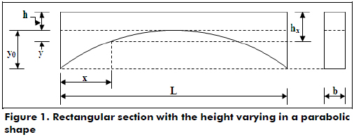
The value "hx" varies with respect to "x", which gives:

Now, the properties of the parabola are used:

Equation (2) is substituted into equation (1):

Derivation of the equations for a uniformly distributed load

Figure 2(a) shows the beam AB subjected to a uniformly distributed load with fixed-ends. The fixed-end moments are found by the sum of the effects. The moments are considered positive in the counterclockwise direction and negative in the clockwise direction. Figure 2(b) shows the same beam simply supported at its ends with the load applied to find the rotations O_A1 and O_B1. Now, the rotations O_A2 and O_B2 are caused by the moment MAB applied at support A, according to Figure 2(c), and in terms of O_A3 and O_B3 are caused by the moment MBA applied at support B, as shown in Figure 2(d) (Przemieniecki, 1985).

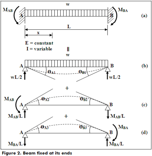
The conditions of geometry are (González Cuevas, 2007; Luévanos Rojas, 2012; Luévanos Rojas, 2013):

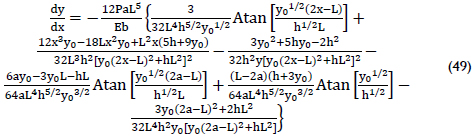
The beam of Figure 2(b) is analyzed to find OA1 and OB1 by Euler-Bernoulli theory to calculate the deflections (Ghali et al., 2003; Mc Cormac, 2007). The equation is:

where dy/dx = Oz is the total rotation around the axis "z"; E is the modulus of elasticity of material; Mz is the moment around the axis "z"; and Iz is the moment of inertia around the axis "z".

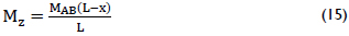
The moment anywhere along the beam on the axis "x" is (Gere et al., 2009):

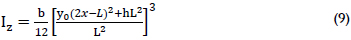
The moment of inertia for a rectangular member is:

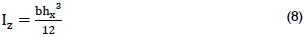
Equation (3) is substituted into equation (8):

Now, equations (7) and (9) are substituted into equation (6):

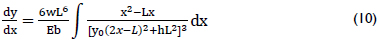
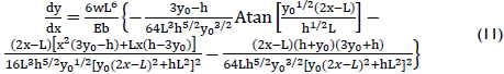
The integral of the equation (10) becomes:

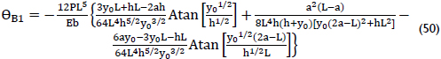
Substituting x = 0 into equation (12) to find the rotation at support A:

Substituting x = 0 into equation (12) to find the rotation at support A:

Substituting x = L into equation (12) to obtain the rotation at support B:

Now, the member of Figure 2(c) is analyzed to find OA2 and OB2 as a function of MAB:

The moment anywhere along the beam on the axis "x" is:

Equations (9) and (15) are substituted into equation (6):

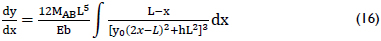
The integral of the equation (16) becomes:

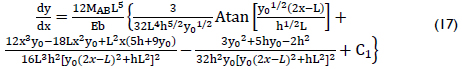
Equation (17) is integrated to obtain the displacements because there are no known conditions for rotations. The equation is as follows:

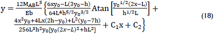
The boundary conditions x = 0 and y = 0 are substituted into equation (18) to find C2:

Then, the boundary conditions x = L and y = 0 are substituted into equation (18) to obtain C1:

Once the constant C1 is obtained, this is substituted into equation (17):

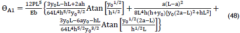
Substituting x = 0 into equation (21) to find the rotation at support A:

Substituting x = L into equation (21) to find the rotation at support B:

Then, the member of Figure 2(d) is analyzed to find OA3 and OB3 as a function of MBA:

The moment anywhere along the beam on the axis "x" is:

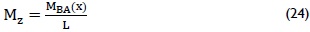
Equations (9) and (24) are substituted into equation (6):

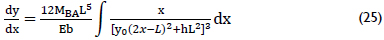
Equation (25) is evaluated in the same manner as Figure 2(c) to find the rotations. They are:

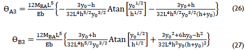
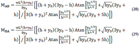
Equations (13), (22) and (26) corresponding to support A are substituted into equation (4), and equations (14), (23) and (27) corresponding to support B are substituted into equation (5). Subsequently, the generated equations are solved to obtain the values of "MAB" and "MBA". These are presented in equations (28) and (29).

Derivation of equations for a concentrated load

Figure 3(a) shows the beam AB subjected to a concentrated load located anywhere along member or fixed-ends. The fixed-end moments are found by the procedure used for the previous case.

The conditions of geometry are shown in equations (4) and (5).

The beam of Figure 3(b) is analyzed to find O_A1 and O_B1 using the Euler-Bernoulli theory to calculate the deflections using equation (6).

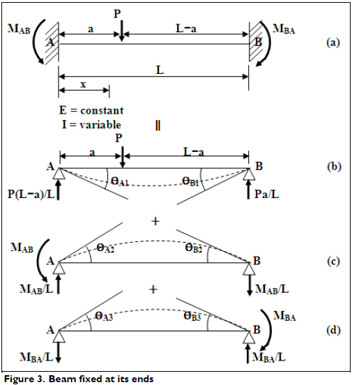
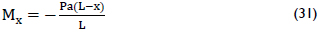
The moment anywhere along the beam on the axis "x" is:

For 0 ≤ x ≤ a

For a ≤ x ≤ L

The moment of inertia for a rectangular member is shown in equation (9).

a) For the portion of the beam where 0 ≤ x ≤ a

Equations (9) and (30) are substituted into equation (6):

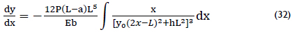
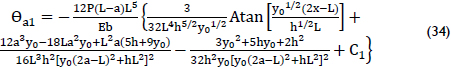
The integral of the equation (32) becomes:

Substituting x = a into equation (33) to find the rotation O_a1:

Equation (33) is integrated to obtain the displacements because there are no known conditions for the rotations:

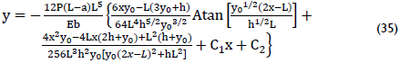
The boundary conditions x = 0 and y = 0 are substituted in equation (35) to find C₂:

Equation (36) is substituted into equation (35):

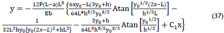
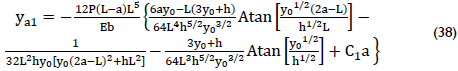
Substituting x = a into equation (37) to find the vertical displacement ya1, where the load P is applied:

b) For the portion of the beam where a ≤ x ≤ L

Equations (9) and (31) are substituted into equation (6):

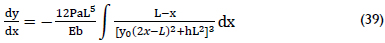
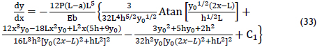
The integral of equation (39) becomes:

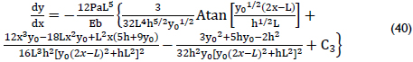
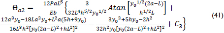
Substituting x = a into equation (40) to find the rotation θ_a2:

Equation (40) is integrated to obtain the displacements because there are no known conditions for rotations:

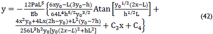
The boundary conditions x = L and y = 0 are substituted into equation (42) to find C₄ as a function of C₃:

Equation (43) is substituted into equation (42) after the boundary condition x = a is included to find the vertical displacement y_a2:

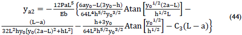
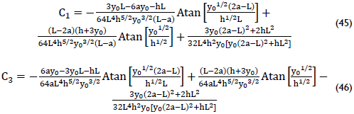
Equations (34) and (41) are equated, as well as equations (38) and (44), because both the rotation and vertical displacement must be equal at the point of application of the load P to find constants C₁ and C₃. These values are:

Equation (45) is substituted into equation (33) to obtain rotations anywhere along the span 0 ≤ x ≤ a:

Substituting x = 0 into equation (47) to find the rotation at support A:

Equation (46) is substituted into equation (40) to obtain rotations anywhere along the span a ≤ x ≤ L:

Substituting x = L into equation (49) to find the rotation at support B:

The member of Figure 3(c) is analyzed to find OA2 and OB2 as a function of MAB. These are shown in equations (22) and (23).

Now the member of Figure 3(d) is analyzed to obtain OA3 and OB3 as a function of MBA. These are presented in equations (26) and (27).

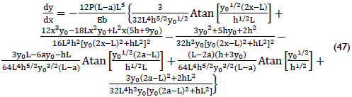
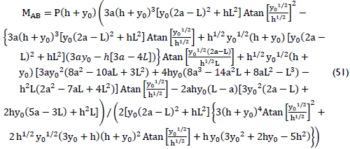
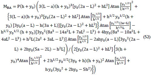
Equations (22), (26) and (48) corresponding to support A are substituted into equation (4), and equations (23), (27) and (50) corresponding to support B are substituted into equation (5). Subsequently, the generated equations are solved to obtain the values of "MAB" and "MBA". These equations are presented in equations (51) and (52).

Results

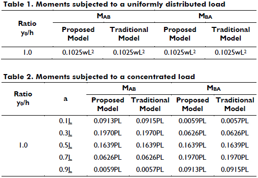
Tables 1 and 2 show comparisons of the two models. The proposed model is the mathematical model developed in this paper, and the traditional model is presented in the tables on page 516 (Hibbeler, 2006). Table 1 shows the moments subjected to a uniformly distributed load, and Table 2 presents the moments subjected to a concentrated load located anywhere along the length of the beam. Such comparisons were determined for a ratio of y₀/h = 1 because these values are presented in the tables mentioned above. The results are virtually identical; therefore the proposed model is valid.

Conclusions

This paper presents a mathematical model for fixed-end moments for two different load types for beams with a parabolic shaped variable rectangular cross section. The loads applied on the beam are: 1) a uniformly distributed load or 2) a concentrated load located at anywhere along the length of the beam. The properties of the rectangular cross section of the beam vary along its axis, i.e., the width "b" is constant and the height "h" varies along the beam in a parabolic form.

The validation of the proposed model is presented by Tables 1 and 2, where the results are virtually identical, but these tables present only the ratio of y₀/h = 1.

The significant advantage of the proposed model is it works for any ratio of y₀/h. Another advantage is in Table 2, where the tables submitted in the books are limited to certain relationships of a = 0.1L, 0.3L, 0.5L, 0.7L, 0.9L, but the model developed in this paper is for any value of "a".

The mathematical technique presented in this research is well suited to obtain the fixed-end moments, rotations and displacements for beams of variable rectangular cross section subjected to a uniformly distributed load or concentrated load because the results are accurate and presented as a mathematical expression.

The application of fixed-end moments, rotations and displacements is significant in the matrix methods of structural analysis to obtain the acting moments and the stiffness of a member.

In addition to the efficiency and precision of the developed model, a significant advantage is that rotations and displacements, as well as the moments, are calculated for any cross section of the beam using the respective integral representations as mathematical formulas.

References

Gere, J. M., & Goodno, B. J. (2009). Mechanics of Materials (7th ed.) (pp. 720-724). New York: Cengage Learning.         [ Links ]

Ghali, A., Neville, A. M., & Brown, T. G. (2003). Structural Analysis: A Unified Classical and Matrix Approach (5th ed.) (pp. 459-505). Taylor & Francis.         [ Links ]

González Cuevas, O. M. (2007). Análisis estructural (pp. 427-437). México: Limusa.         [ Links ]

Hibbeler, R. C. (2006). Structural analysis (6th ed.) (pp. 503-520). New Jersey: Prentice-Hall, Inc.         [ Links ]

Luévanos Rojas, A. (2012). Method of structural analysis for statically indeterminate beams. International Journal of Innovative Computing, Information and Control, 8(8), 5473-5486.         [ Links ]

Luévanos Rojas, A. (2013). Method of structural analysis for statically indeterminate rigid frames. International Journal of Innovative Computing, Information and Control, 9(5), 1951-1970.         [ Links ]

Mc Cormac, J. C. (2007). Structural analysis: using classical and matrix methods (pp. 550-580). New York: John Wiley & Sons.         [ Links ]

Przemieniecki, J. S. (1985). Theory of Matrix Structural Analysis (pp. 150-163 and 278-287). New York: McGraw-Hill.         [ Links ]

Tena Colunga, A. (2007). Análisis de estructuras con métodos matriciales (pp. 101-102). México: Limusa-Wiley.         [ Links ]

Vaidyanathan, R., Perumal, P. (2005). Structural Analysis (Vol. I)( pp. 38-40). New Delhi: Laxmi Publications (P) LTD.         [ Links ]

Williams, A. (2008). Structural Analysis (pp. 273-275 and 315). New York: Butterworth Heinemann.         [ Links ]