http://dx.doi.org/10.15446/ing.investig.v34n2.40596

S. Diez¹, E. Barra², F. Crespo³ and J. Britch⁴

¹ Sebastian Diez. Chemical Engineer, MSc in Environmental Engineering, Universidad Tecnológica Nacional (UTN-FRC), Argentina. Affiliation: Centro de Investigación y Transferencia en Ingeniería Química Ambiental (CIQA), UTN-FRC, Argentina. E-mail: sdiez@ciqa.com.ar

² Enrique Barra. Chemical Engineer Student, UTN-FRC, Argentina. Affiliation: CIQA, UTN. E-mail: enriquebarra@live.com.ar

³ Flavia Crespo. Chemical Engineer Student, UTN-FRC, Argentina. Affiliation: CIQA, UTN. E-mail: flaviacrespo@live.com.ar

⁴ Javier Britch. PhD en Phisics, Universidad Nacional de Córdoba, Argentina. Affiliation: CIQA, UTN-FRC. E-mail: javierbritch@hotmail.com

How to cite: Diez, S., Barra, E., Crespo, F., & Britch, J. (2014). Uncertainty propagation of meteorological and emission data in modeling pollutant dispersion in the atmosphere. Ingeniería e Investigación, 34(2), 44-48.

ABSTRACT

Variability is true heterogeneity existing within a population that cannot be reduced or eliminated by more or better determinations. Uncertainty represents ignorance about poorly characterized phenomena, but it can be reduced by collecting more data. The aim of this paper was to study the impact of the variability and uncertainty of the main variables, i.e., emissions and meteorology, of the PM10 concentration caused by a point source located at Malagueño (Córdoba, Argentina). To perform this analysis, a scheme was developed using the USEPA Industrial Source Complex model algorithms with a Monte Carlo methodology. Using a simulation with one hundred thousand iterations, the concentration distribution was obtained and showed that the uncertainty in wind direction had the greatest impact on the estimates.

Keywords: Uncertainty, Variability, Monte Carlo, PM10.

RESUMEN

La variabilidad es la heterogeneidad real dentro de una población, que no puede ser reducida ni eliminada por más o mejores determinaciones. La incertidumbre representa la ignorancia acerca de un fenómeno pobremente caracterizado, pero que puede reducirse mediante la recopilación de más datos. El objetivo de este trabajo es estimar la concentración de PM10 provocada por las emisiones de una fuente puntual ubicada en Malagueño (Córdoba, Argentina), considerando la variabilidad y la incertidumbre de la meteorología y las emisiones. Para abordar este análisis fue desarrollado un método que utiliza los algoritmos del modelo Industrial Source Complex de la USEPA junto a la metodología Monte Carlo. Con cien mil iteraciones se obtuvo la distribución de concentraciones, encontrándose que la incertidumbre en la dirección del viento es la de mayor incidencia sobre las estimaciones.

Palabras clave: Incertidumbre, Variabilidad, Monte Carlo.

Received: November 1th 2011 Accepted: February 25th 2014

Introduction

Atmospheric dispersion models are tools used for predicting the fate and transport of air pollutants to assess the impact of emission sources on air quality (Monteiro et al., 2008). However, because atmospheric dispersion is a stochastic phenomenon, the concentration at a given time and place cannot be predicted accurately (Chatwin, 1982). In addition to the inherent uncertainty and variability of atmospheric processes, there are also errors associated with the air quality models and the parameters used (Hanna et al., 1998). Examples of these are errors associated with the input data, the use of surrogate data, the model formulation and its subsequent application outside its validity range. While variability is the true heterogeneity observed in nature (with temporal, spatial or inter-individual differences), uncertainty is defined as the incomplete knowledge of a specific magnitude whose "real value" could only be established if there were a perfect measuring device (Cullen and Frey, 1999). Variability is a property of the system under study and cannot be reduced even by improving the measurement system. In contrast, uncertainty is considered to be a property of the measurement process and can be minimized, for example, by obtaining more data or higher quality data (Dabbberdt and Miller, 2000).

Baumann-Stanzer and Stenzel (2011) quantify the effects of meteorological uncertainties over hazard distances using different models for scenarios with chlorine, ammoniac and butane. Hanna et al. (2007) analyze the effects of emissions, meteorological and dispersion model parameter uncertainties over the annually averaged concentrations of benzene and 1,3-butadiene estimated with ISC3 and AERMOD models with the Monte Carlo method. Yegnan, et al. (2002) calculate the uncertainty in ground-level concentrations of ISCST calculations using first- and second-order Taylor series. Garcia-Diaz and Gozalvez-Zafrilla (2012) applied uncertainty and sensitivity analysis methods over the ISC3 model to analyze the influences of wind speed, wind direction, and pollutant emission rate to predict the ground-level concentration of sulfur dioxide emitted by a power plant.

The aim of this work was to evaluate the uncertainty in the estimation of the PM10 concentration (particulate matter ≤ 10 microns), which contributes to the ambient value, associated with a point source located 2 km south of Malagueño City (Province of Córdoba, Argentina). Here, only one source of uncertainty was considered: the dispersion model input data. This type of uncertainty includes systematic errors or biases in the data collection process, imprecision in analytical measurements, inference due to limited data or an unrepresentative variable, as well as the extrapolation or use of surrogate data for the parameters of interest.

The variables analyzed were meteorological variables (wind speed and direction, atmospheric stability and temperature) and emissions variables (exhaust temperature, emission rate, and exhaust velocity). The meteorological variables were obtained from the National Meteorological Service, and the emission variables were estimated by evaluating the specific factors of industrial processes. To address this problem, the ISC (Industrial Source Complex) (EPA, 1995) dispersion model was used in conjunction with the Monte Carlo simulation (MC).

Materials and Methods

Dispersion Model

From the wide variety of mathematical tools available for dispersion modeling (lagrangian, Eulerian, grid models, etc.), a Gaussian model application, the ISC3 computational model (EPA, 1995a), was chosen due to its simplicity and low computational costs. ISC3 is a steady-state Gaussian Plume Model that was created by the U.S. Environmental Protection Agency (EPA) for regulatory purposes. It was the preferred EPA model before being superseded by AERMOD (EPA, 2005) in 2006. Thereafter, ISC has been known as an "alternative model", despite its current use as a regulatory model in many parts of the world, as a result of its robustness, adaptability to different situations, availability of required data and relative ease-of-use compared to more advanced models.

Uncertainty propagation: Monte Carlo Simulation

The steps usually followed in the MC simulation are (i) identify the mathematical model that best represents the system under study, (ii) describe the probability distributions of the variables of the model, (iii) take random samples from different distributions that characterize the input data, and (iv) obtain the output value set by the mathematical model for each sample. Finally, statistical analysis is performed on the output values to support decision making (Glasserman, 2003). The minimum number of iterations in a MC simulation depends on the quantity of input parameters (and whether they are correlated or not) and the confidence required in the output probability distribution (Graettinger and Dowding, 2001). Although other methods exist, the most direct route for generating a random sample from a given distribution is the inverse method (Raychaudhuri, 2008). This scheme uses the inverse of the cumulative distribution function by converting a random number between 0 and 1 to another random value of the input distribution. As a rule of thumb, the model must be run a sufficient number of times to achieve numerical stability in the distribution tail.

Emission source characterization

The emission source used as the application case belongs to a cement plant located in Malagueño (Province of Cordoba). Currently, in this town, there are several activities related to lime mining and its industrialization. These operations emit particulate matter that can affect human health, primarily the respiratory system (WHO, 2005). The particulate source analyzed uses a so-called "dry process" for the production of cement. Prior to emission in the atmosphere, the combustion gases are filtered using a baghouse filter.

Emission rates are normally determined by continuous or periodic emission monitoring using material balances or through emission factors derived from similar sources. In our case, there were no monitoring data and no access to the process material balance; emission factors for PM10 were estimated using the AP-42 guidance (EPA, 1995b). According to Schvarzer and Petelski (2005), the production of this plant (its activity rate) in 2005 was 1.5 x 106 tons of cement, which resulted in an emission rate of 4.75 g/s. Although the current production is unknown, it was reported that, in 2005, the consumption of cement in Argentina was 9 x 106 tons (Farfaro Ruiz, 2010); 11.5 x 106 tons were sold by late 2012. Assuming a linear relationship exists in recent years between the consumption and the production of cement in Argentina (Farfaro Ruiz, 2010), it was estimated that the Malagueño plant could be producing 1.9 x 106 tons, resulting in an emission rate of 6.02 g/s of PM10 in 2012.

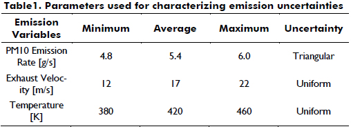
Because knowledge of the behavior of the emission variables was limited, probability distributions of a minimum complexity were used. Based on this, the values utilized were the upper and lower limits with the mean value considered to be the most likely value of a triangular distribution. The exhaust velocity and temperature of the gases were taken from the description of similar processes (Schneider et al. 1996; EQM 2008; EC, 2000; NEPA, 2004), which employed ranges to describe these variables. The following table summarizes the values used:

Characterization of meteorology

Meteorological data are the cause of more than half of the uncertainty in predicting hourly concentrations with dispersion models (Rao, 2005). In addition to the natural variability of the atmosphere, the use of meteorological data taken at non-representative locations, the use of inappropriate instruments or non-systematic recording and data storage are some of the most influential factors affecting a dispersion model's uncertainty.

For the present study, 5 years of consecutive data (2007-2011) were provided by the National Weather Service (NWS) and measured at Ambrosio Taravella International Airport (approximately 20 km from the application zone). These data correspond to wind speed, wind direction, ambient temperature and atmospheric stability.

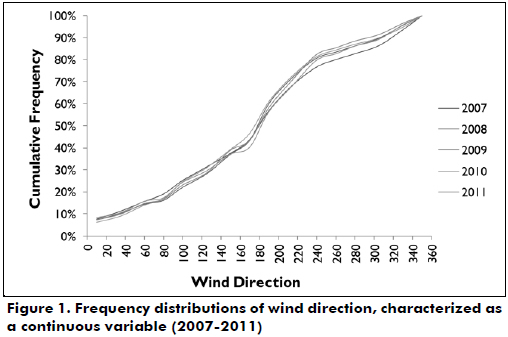
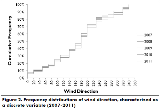
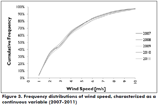
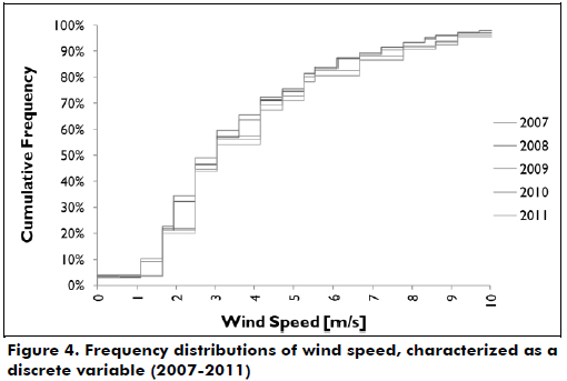
Two of the variables provided by the NWS (i.e., wind speed and direction) are characterized by discrete jumps. These discontinuities may be caused by the sensitivity of the measuring instruments, the methodology used for the processing of measurements and how the data are "packaged" for distribution. This characteristic generates uncertainty of the "true" distribution of both variables because they are continuous variables. Therefore, the measurement and recording of these variables generated an intra-range uncertainty, and consequently, both wind direction and wind speed were first characterized as continuous variables and then as discrete variables to assess the impact on the estimated PM10 concentration. The distributions for wind speed and direction are shown in Figures 1 to 4. Additionally, the effect of the interannual variation of the meteorology was also taken into account by using each of the five years independently to obtain more robust confidence intervals.

Results

Variability and uncertainty

The variability and uncertainty analysis was performed over the maximum exposed receptor (MER). To determine the MER, EPA's ISC model was run. The urban area of Malagueño was represented by a 36 km² grid (with the origin at the point source) and a total of 931 nodes every 200 meters. Furthermore, the study area was considered rural because less than 50% of the area of influence (determined by a circle with a 3 km radius that was centered on the point source) is industrial, commercial or residential (EPA, 2005).

Then, the Monte Carlo method was applied. Two runs per year (for a total of 10 runs) were performed: the first run with wind speed and wind direction as "continuous" and the second run with wind speed and wind direction as "discrete" while maintaining the rest of the atmospheric variables (temperature and stability) under the same characterizations. Each simulation for the MER was performed with 1x10⁵ iterations. The simulations for each of the 10 scenarios were constructed using the uncertainty bands shown in Figure 5. Specifically, for each scenario, a distribution of concentrations (response distribution) was calculated. With these 10 response distributions, the confidence limits were estimated. The "y" axis is the cumulative frequency, now named the "variability percentile". This naming convention helps to distinguish the empirical frequency distributions of the input variables and the output (concentration) percentiles estimated with the Monte Carlo method. Second, it emphasizes the fact that this axis shows the temporal variability on the MER.

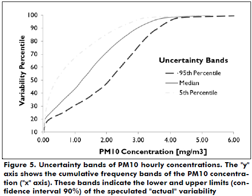
As can be observed in fig. 5, the uncertainty bands are wider between the 30th and 90th percentiles, whereas the bands became closer in the lower and higher percentiles.

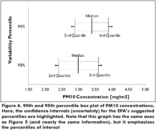
According to the EPA (USEPA, 2002), decisions regarding the management of health risks should be based on the worst case scenario. If sufficient information exists (e.g., to build probability distributions), decisions may be based on the tail of the distribution (e.g., 90th or 95th percentiles). Following EPA suggestions, Figure 6 shows the confidence intervals (uncertainty) at the 90th and 95th percentiles of concentration's variability.
From this figure, it can be argued with 90% confidence (width of the confidence interval) that 90% (i.e., 90th percentile) of the PM10 hourly average concentration did not exceed 3.62 g/m³; 2.97 mg/m³ is the most likely value for this percentile. In addition, the 95th percentile of the PM10 average hourly concentration (90% confidence) did not exceed the value of 3.94 g/m3, with a median value of 3.39 g/m³.

Sensitivity

Sensitivity analysis evaluates how the change in a model's output variables can be attributed, qualitatively or quantitatively, to different sources of variation in the input data (Saltelli et al., 2008). In Figure 7, the Spearman correlation coefficient is shown; it takes into account the behavior of the 50th and 95th concentration percentiles. The emission variables (PM10 emission rate, exhaust velocity and temperature) are grouped under one label due to their joint effect on sensitivity.

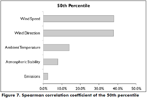
The variables with the greatest impact on the median (50th percentile) were the meteorological variables, primarily wind speed and wind direction, followed by the ambient temperature and stability. The set of emission variables (emission rate, speed and gas temperature) had the lowest impact.

Given the implications for decision making, what is observed in the 95th percentile (distribution tail) is very important. In this percentile, the wind direction was the variable with the greatest impact. In contrast with the 50th percentile, the second most influential variable was the uncertainty introduced by the emissions and was, to an extent, similar to the wind speed, atmospheric stability and ambient temperature with the lowest impacts.

Conclusions

The concentration of PM10 (and any other air pollutant concentration) is a random variable that cannot be predicted accurately, but it can be described using a probability distribution, which provides a better understanding of the concentration. A deterministic estimate does not provide complete information of the scenario because the concentration's uncertainty is not considered. For that reason, ISC3 (and other regulatory models) should be modified to accept uncertainties as input data and to report estimated concentrations along with its uncertainties. This could be used to allow decision makers to evaluate the validity of these estimates in actual applications. For example, if the lower confidence limit value (5th percentile) was above a regulatory standard, then corrective/preventive actions will most likely be needed. If the upper confidence limit (95th percentile) was below the standard, then corrective/preventive measures will most likely not be required. Thus, dispersion modeling supported by an uncertainty analysis could provide an important tool for decision making.

Modeling the dispersion of air pollutants requires a large number of inputs, some of which are subjected to large uncertainties. Additionally, assumptions often have to be made that tend to overestimate the actual concentrations.

In this work, the variability and uncertainty in PM10 concentration modeling was estimated using a point source located in Cordoba Province as a case study. Two main sources of uncertainty were considered: meteorology and emissions.

The meteorology data used presented discrete jumps in wind speed and wind direction, even though both variables are continuous. Therefore, the propagation of this source of uncertainty was analyzed considering (i) continuous probability functions and (ii) discrete probability functions.

The AP-42 method was used for the estimation of the emission factors, which also introduced uncertainties into the calculations; however, these uncertainties were not considered here because, according to our criteria (uncertainty is a property of the analyst), this uncertainty is overlapped by the uncertainty in the activity rate given that there are not recent, available data.

Five years of meteorological data were fitted to several distributions, and 10 runs (two runs per year) were performed (1x10⁵ iterations each) with the support of the ISC3 model combined with Monte Carlo. Ten PM10 concentration distributions were obtained for the maximum exposure receptor.

By defining wind speed and direction with discrete distributions, it was observed that higher concentrations were produced with respect to their counterparts, resulting in very large uncertainty bands between the 30th and 90th percentiles. With a 90% confidence, the 90th and 95th percentiles were 3.62 ug/m³ and 3.94 ug/m³, respectively.

Through sensitivity analysis, it was determined that the direction and emission variables were the most important factors affecting the uncertainty in the distribution tail. With these findings, it can be concluded that by obtaining higher quality data (wind speed, wind direction and emission variables), the uncertainty bands will decrease dramatically and thus improve the quality of the estimations made with the ISC3 dispersion model.

Finally, it is important to note that although there are other meteorological and emission variables subject to uncertainties (e.g., roughness length, mixing height, precipitation, cloud cover, ceiling height, and emission factor), they were not considered here. Otherwise, it would be important to study the implications of these factors' uncertainties in the dispersion modeling.

References

Abdul-Wahab, S. A. (2006). Impact of fugitive dust emissions from cement plants on nearby communities. Ecological Modelling, 195(3-4), 338-348.         [ Links ]

Baumann-Stanzer, K., & Stenzel, S. (2011). Uncertainties in modeling hazardous gas releases for emergency response. Meteorologische Zeitschrift, 20(1), 19-27.         [ Links ]

Curtis, L., Rea, W., Smith-Willis, P., Fenyves, E., & Pan, Y. (2004). Adverse health effects of outdoor air pollutants. Environment international, 32(6), 815-830.         [ Links ]

Dabberdt, W. F., & Miller, E. (2000). Uncertainty, ensembles and air quality dispersion modeling: Applications and challenges. Atmospheric Environment, 34(27), 4667-4673.         [ Links ]

Department of the Environment, Water, Heritage & the Arts. National Pollutant Inventory: Emission estimation technique manual for cement manufacturing, 2008. Australian government. Retrieved from http://www.npi.gov.au/publications/emission-estimation-technique/pubs/cement.pdf         [ Links ]

Donnelly, R. P., Lyons, T. J., & Flassak, T. (2007). Evaluation of results of a numerical simulation of dispersion in an idealized urban area for emergency response modelling. Atmospheric Environment, 43(29), 4416-4423.         [ Links ]

Environmental Protection Agency (1995). User's Guide for the Industrial Source Complex (ISCST3) Dispersion Models. Description of model algorithms (Vol. 2). Retrieved from http://www.epa.gov/scram001/userg/regmod/isc3v2.pdf        [ Links ]

Environmental Protection Agency (1995). Compilation of Air Pollutant Emission Factors, Volume 1: Stationary Point and Area Sources. Office of Air Quality Planning and Standards. Retrieved from http://www.epa.gov/ttnchie1/ap42        [ Links ]

Environmental Protection Agency (2005). Revision to the Guideline on Air Quality Models: Adoption of a Preferred General Purpose (Flat and Complex Terrain) Dispersion Model and Other Revisions. Retrieved from http://www.epa.gov/scram001/guidance/guide/appw_05.pdf        [ Links ]

Garcia-Diaz, J. C., & Gozalvez-Zafrilla, J. M. (2012). Uncertainty and sensitive analysis of environmental model for risk assessments: An industrial case study. Reliability Engineering and System Safety, 107, 16- 22.         [ Links ]

Ghannam, K., & El-Fadel, M. (2013). Emissions characterization and regulatory compliance at an industrial complex: an integrated MM5/CALPUFF approach. Atmospheric Environment, 69, 156-169.         [ Links ]

Ghenai, C., & Lin, C. (2006). Dispersion Modeling of PM10 Released during Decontamination Activities. Journal of Hazardous Materials, 132(1), 58-67.         [ Links ]

Hanna, S. R., Paine, R., Heinold, D., Kintigh, E., & Baker, D. (2007). Uncertainties in Air Toxics Calculated by the Dispersion Models AERMOD and ISCST3 in the Houston Ship Channel Area. Journal of Applied Meteorology and Climatology, 46, 1372-1382.         [ Links ]

Kiely, G. (1999). Environmental Engineering. International edition. McGraw-Hill Higher Education.         [ Links ]

Krupa, S., O'Neill, S., Faulkner, B., & Shaw, B. (2009). Differences in the Chemical Composition of Particulate Matter (PM) by their Size and their Importance in Ambient Sampling of PM. Retrieved from ftp://ftp-fc.sc.egov.usda.gov/AIR/AAQTF/200809-201009/200909_DesMoines_IA/AAQTF_200909_AQ_StdsSubcommittee_whitepaper.pdf        [ Links ]

Pérez Camaño, J. (2004). Sistema integrado para la modelización and el análisis de la calidad del aire en modo operacional (Unpublished doctoral dissertation). Universidad Politécnica de Madrid. Madrid, España.         [ Links ]

Rao, K. S. (2005). Uncertainty Analysis in Atmospheric Dispersion Modelling. Pure and Applied Geophysics, 162, 1893-1917.         [ Links ]

Schvarzer, J., & Petelski, N. C. (2005). La industria del cemento en la Argentina. Un balance de la producción, la capacidad instalada y los cambios empresarios, tecnológicos y de mercado durante las últimas dos décadas. Retrieved from http://www.jorgeschvarzer.com.ar/info/pdf_web/2005/documento-de-trabajo-n.-8-la-industria-del-cemento-cespa.pdf        [ Links ]

Sincich, S., & Maggi, R. (2008). Prácticas culturales de recuperación documental: el archivo histórico de la Municipalidad de Malagueño. Municipio de Malagueño, Provincia de Córdoba. Retrieved from http://www.mundoarchivistico.com/?menu=articulos& id=116        [ Links ]

World Health Organization. Particulate matter air pollution: how it harms health, 2005. Retrieved from http://www.chaseireland.org/Documents/WHOParticulateMatter.pdf        [ Links ]

World Health Organization. Air quality guidelines for particulate matter, ozone, nitrogen dioxide and sulfur dioxide. Summary of risk assessment, 2006. Retrieved from http://whqlibdoc.who.int/hq/2006/WHO_SDE_PHE_OEH_06.02_eng.pdf         [ Links ]

Yang, C., Chang, C., Tsai, S., Chuang, H., Ho, C., Wu, T., & Sung, F. (2003). Preterm delivery among people living around Portland cement plants. Environmental Research, 92(1), 64-68.         [ Links ]

Yegnan, A., Williamson, D. G., & Graettinger A. J. (2002). Uncertainty analysis in air dispersion modeling. Environmental Modelling & Software, 17(7), 639-649.         [ Links ]