DOI: http://dx.doi.org/10.15446/ing.investig.v34n3.41943

J. D. Rairán¹

José Danilo Rairán Antolines. Electrical Engineering, Industrial Automation Magister, Ph. D. Candidate, Universidad Nacional de Colombia, Colombia. Affiliation: Universidad Distrital Francisco José de Caldas, Colombia. E-mail: drairan@udistrital.edu.co

How to cite: Rairán, J. D. (2014). Two Algorithms for Estimating the Period of a Discrete Signal. Ingeniería e Investigación, 34(3), 57-63.

ABSTRACT

In this paper, we present two algorithms for approximating a period given a discrete data set. These algorithms superimpose two consecutive sections of the data for several candidate periods. The first algorithm counts the number of shuffling points per candidate period, whereas the second algorithm computes a distance between points when sorted by time. The best candidate period maximizes the number of shuffling points in the first algorithm, whereas the second algorithm minimizes the distance between points. The experimental validation with noiseless data demonstrates that the relative error for the estimations is less than half of the sampling period and shows that this error does not depend on the harmonic content, as normally occurs with algorithms that estimate a period. The application of the algorithms demonstrates that they properly track the frequency of a power grid and accurately estimate the period of a Van der Pol oscillator, which serves to confirm their applicability to real-time problems.

Keywords: Frequency estimation, frequency measurement, periodic functions, power system monitoring, signal reconstruction.

RESUMEN

En este artículo se presentan dos algoritmos para estimar el periodo de una señal, dado un conjunto de datos discretos, estos algoritmos superponen dos secciones de datos a varios periodos. El primer algoritmo cuenta el número de puntos que se mezclan por cada periodo, mientras el segundo, calcula la distancia entre los puntos cuando se ordenan por tiempo. De esta manera, el mejor candidato para periodo maximiza el número de puntos que se mezclan en el primer algoritmo, mientras que en el segundo, minimiza la distancia entre puntos.

La validación experimental con señales sin ruido, demuestra que el error relativo de las estimaciones cae por debajo de la mitad del periodo de muestreo, y a su vez, muestra que ese error no depende del contenido armónico de la señal, como ocurre con los algoritmos para estimar periodo. La aplicación de los algoritmos demuestra que pueden seguir la frecuencia de un sistema de potencia y además, pueden aproximar el periodo de un oscilador Van der Pol, lo cual sirve para confirmar que estos algoritmos se pueden aplicar para solucionar problemas en tiempo real.

Palabras clave: estimación de frecuencia, medida de frecuencia, funciones periódicas, monitoreo de sistemas de potencia y reconstrucción de señales.

Received: February 6th 2014 Accepted: August 18th 2014

Introduction

The discretization performed by an electronic device to record samples of an analog signal depends on the device's memory, the frequency of its internal clock, and the required precision. However, in general, it does not depend on the period of the signal itself because this value almost always remains unknown. Thus, generally speaking, the measurement of discrete signals produces data points that do not match the period of the signal, and consequently, the computation of the period results in a mere approximation of the true value. The inevitable errors that occur when estimating a period influence a wide variety of processes, such as signal reconstruction and prediction.

Given the availability of several methods for reconstructing a signal given its period and given appropriate data sampled at an appropriate rate (Petrovic and Stevanovic, 2011), the problem consists of estimating the period of a signal or, equivalently, approximating its fundamental frequency. Current work in frequency estimation focuses on sinusoidal signals, whereas the approach in this paper extends the estimations to a broader family of functions: functions of bounded variation. One example is the method of phase unwrapping, which estimates the frequency by performing a linear regression on the phase of the signal (McKilliam et al., 2010). However, this method cannot be used in real-time applications due to its high computational requirements. Another method guarantees results for noiseless conditions and bases its results on the solution of a system of linear equations using a DFT for two time intervals (Provencher, 2010). In contrast, So and Chan combine a matrix of elements converted to two unitary vectors to provide an estimate of the frequency, but their algorithm requires an iterative process (So, Chan, and Weize, 2011). Other approaches allow several sinusoidal components. One approach minimizes the mean squared error between an assumed signal model and the actual signal to estimate the frequency of a power system (Chudamani, Vasudevan, and Ramalingam, 2009). This last approach focuses on methods that can be implemented in electronic circuits, but the methods neither guarantee the performance nor compare the performance of their algorithm with popular estimators. Pantazis and colleagues (2010) suggest a time-varying sinusoidal representation to estimate frequencies for various signals such as speech and audio signals. The experimental results show that the suggested algorithm outperforms FFT-based approaches in non-stationary environments. Finally, a more general family of algorithms uses the DFT as a basis for estimating frequencies. For instance, a method exclusively used for complex exponential waveforms in the presence of white noise uses DFT in the first stage, after which the three terms with the highest spectral magnitudes produce a better estimate (Candan, 2011). Candan claims that the estimation performs well for small and medium sampling rates, but nothing is said about high sampling rates. Yang and Wei (2011) present a non-iterative method consisting of two parts: a coarse estimation, given by the FFT, and a fine estimation, using least squares minimization of three spectral lines.

The contribution of this paper consists in the presentation of two new algorithms for approximating a period given a discrete data set. Some of the main advantages include the lack of assumptions about the number of data points and the independence of the harmonic content, as clearly shown by comparisons with the most common method used to approximate a period: the periodogram (Ta-Hsin and Kai-Sheng, 2009). The approximations depend exclusively on the distance between the last data point before the period and the period itself. However, requirements on the data set and the use of iterations to produce an estimate may make the algorithms computationally expensive.

The following section studies the periodogram as a method for approximating a period and focuses on the error in its estimations. Then, for all of the algorithms, Section 3 analyzes the effects of having errors in an estimated period, which subsequently justifies, in Section 4, the introduction of the new algorithms to reduce the errors. Then, Section 5 presents an evaluation of the quality of the approximations for the new algorithms given noiseless and noisy data. Once the experimental evidence validates the algorithms, Section 6 details two examples that show the applicability of the proposed methods. Finally, Section 7 presents the conclusions and discusses future work.

Approximation of a period by a periodogram

This section analyzes the error of approximating the period by a method known as the periodogram. This method has become a reference for comparing algorithms in terms of the estimation of a period from discrete signals. A periodogram uses equally spaced samples from a signal, producing a candidate period based on the harmonic decomposition of the signal (computed by a Fast Fourier Transform) (Stoica and Moses, 2005). This candidate has a period that is equal to the inverse frequency of the harmonic with the highest magnitude (Ta-Hsin, 2013). Thus, the periodogram assumes that the signal's fundamental harmonic has the maximum amplitude across the whole frequency spectrum. Another strong assumption states that the sampling time should assure the acquisition of a number of data points per period that is equal to an integer power of two; otherwise, the method does not guarantee results.

A group of 25 discrete functions served to test the periodogram method. The results with these functions allowed us to classify the functions into three sets according to the error, which indicates the quality of the approximation. The error corresponds to the difference between a true period (T) and its approximation (T*) relative to the sampling period. The first set of functions decreases the relative error as the length of the data (N) increases. This set will be labeled as a group of "friendly" functions because they satisfy all the assumptions required for the periodogram. A triangular function and a sine function with low harmonic content belong to this first set. The second group, "tractable" functions, is composed of functions that exhibit a behavior that is similar to the first group, but some zones, which may be small, present errors that are greater than one. The third group, "hard" functions, contains functions in which the error is never less than one regardless of the value of N. This behavior may be explained by a failed assumption of the periodogram. The following sections use the six representative functions for the three sets to study the influence of the error in the approximation on the reconstruction of a signal.

All 25 functions have two features in common: they have no noise in the data points, and their mean value equals zero. The noise-free characteristic facilitates the analysis, whereas a null mean value avoids having candidate periods equal to infinity, which results from a zero frequency component as the highest magnitude in the spectrum.

An example of the error surface shown in Figure 1 shows the relative error when approximating a triangular function (a friendly function) for eight points in the first period. In addition to the N axis in the figure, the second axis, ΔN, represents the distance between the last data point before the period and the period itself relative to the sampling period. Thus, 0 ≤ ΔN < 1. This ΔN parameter proved relevant because an assumption of the Fast Fourier Transform is that a data point always matches the period; therefore, ΔN is presumed to always equal zero, which in general proves false. The error when estimating a period finds its source precisely in the existence of this ΔN.

The relative error in the upper part of Figure 1 decreases as N increases, but it does not become less than 1 before N = 32. Specifically, the periodogram requires data equivalent to at least 4 periods (given eight points per period) to have a relative error of less than one. The intermediate plot in Figure 1 presents the maximum error for each N, regardless of ΔN. This plot demonstrates a step behavior, jumping when N becomes equal to a power of two. The lower panel of Figure 1 shows a bell shape for the error. This shape decreases its magnitude and augments its quantity as N increases.

Experimenting with friendly and tractable functions confirms that a periodogram may require a large amount of data to estimate a period with relative errors of less than one. The example in Figure 1 needs four periods, but this requirement may grow to fifty or even hundreds when N does not match 2k, with k being a natural number. In general, larger values of N for a period require a larger number of periods in the data set to produce estimations with an error of less than one.

Effects of the errors on the estimation of a period

This section studies some effects of having errors in the estimation of a period, which justifies the presentation of two new algorithms for approximating a period in the next section. The results come from worked performed in Matlab by the authors using the three families of functions defined in the previous sections.

Influence on Fourier coefficients

This section studies the effects of approximating a period on the values of the coefficients in a Discrete Fourier expansion. The range for the period estimation reaches ±5% of the true period, where T equals 2π. This range exceeds the errors given by a periodogram for the friendly and tractable functions. Thus, the range guarantees the generality of the results in this section. Therefore, given an estimated period, the process consists in computing the Fourier coefficients and subsequently comparing them with a reference, which corresponds to the coefficients computed for the continuous version of each trial function at the true period.

The preliminary results show that, given the trial functions, ΔN does not have any influence on the values of the approximated coefficients. The error surface proved to be completely defined as a function of variations in N and in the estimated period, as illustrated in Figure 2 The results also show that given an approximation (T*) equal to T, increases in N reduce the difference between the approximated coefficients and their continuous versions. This effect becomes visible via the depression in Figure 2 Another major effect allows us to state that underestimating the period may imply lower errors in the coefficient computation compared to overestimating the period, especially for a small number of points, such as less than a hundred points, as shown in Figure 2 This feature becomes evident by observing the depression in the error surface at the left side of the figure. This effect may be explained, in part, by the shapes of the functions. Overestimating a period may induce jumps in the function at the true period, whereas underestimating the period, in general, preserves the main features of the function, which are correlated with the coefficient values.

Influence on signal reconstruction

Consider a continuous function with errors in the estimation of its period. Likewise, suppose that we have an analog reconstruction of that function coming from the approximation given by the expansion of the Fourier coefficients at the estimated period. Now, because of computational requirements, the comparison between the reference function (f) and its reconstruction (f*) uses a sampling equal to five thousand data points per approximated period instead of the continuous version of each function. The measure of quality for the approximation (root mean squared error - rmse) helps us study the effect of errors on the period estimation as well as analyze the effect of different numbers of harmonics on the reconstruction.

The error in signal reconstruction inherits some properties from the approximation of the Fourier coefficients because the reconstruction considered in this section uses a number of Fourier coefficients to reconstruct a signal. However, some features of the errors result from the reconstruction itself and not by inheritance. For instance, the process of signal reconstruction by Fourier coefficients generates equal approximations at the initial and final ends of a period interval. As a result, increasing the number of harmonics as well as the number of data points N may not result in the rmse converging to null.

Influence on electrical energy computation

The negative effects of misleading signal reconstructions can impact a large variety of areas, with implications of varying degrees of seriousness. Among them, computations concerning energy may be some of the most extreme examples because of their consequences to consumers and generators. Any deviation from the true value implies that electrical companies either lose money or are billed for more electricity than what is actually generated, with opposite effects for the consumers.

Measuring electrical energy requires the precise sampling of voltage and current over time, which can be performed by electrical devices based on electromagnetic principles (Bernieri et al., 2010) or by reconstructing voltage and current signals using samples, as is performed by static meters (Berrieri, et al., 2012). This section, to analyze effects on energy computation, supposes an ideal load of 1 ohm, and f = 60 Hz. Thus, the analysis starts by defining an approximated period, with errors from -5% through 5%, whereas the true period equals 1/60 of a second, which are greater than normal deviations in power grids. The next step involves an approximation of the Fourier coefficients, from which the current and voltage signals are reconstructed. Finally, the approximated transmitted energy compared with the true transmitted energy serves as a measure of error.

The first experimental observation, performed at T* equal to T, shows that greater numbers of harmonics and data points per period, in general, better approximate the transmitted energy. Similar results, computed at approximated periods T* different from T, show that increasing N when approximating the coefficients, or increasing the number of harmonics when reconstructing a signal, generally improves the quality of the approximation. In addition, some trial functions display increases in the approximated energy for underestimations of the period, whereas others show the opposite behavior. Thus, the error in the energy computation given an estimated period T* cannot be generalized, and every function requires its own analysis. However, an extreme case in the experiment exhibited an error of 78% in the energy computation at 5% error in the period.

Two new algorithms for estimating a period

Because of the errors generated in the estimation of a period, as was explained using a periodogram, and also given the effect of these errors on signal reconstruction, as discussed in the previous section, this section proposes two algorithms for improving the estimation process. The first part of this section defines the problem, and the second part presents the variables, the algorithms, and a concept of error. This section concludes with a brief example of both algorithms approximating a period.

Problem definition

This paper only concerns the so-called functions of bounded variation over a finite interval. They include the usual signals describable by smooth functions but do not include all continuous functions. However, they include large families of discontinuous functions.

Definition. A function f : [a,b] → R is of bounded variation, denoted f ∈ BV[a,b], if there exists some constant M such that ∑ |f(t_i) - f(t_i+1)| ≤ M (the summation goes from i = 0 to n) for every partition π of a finite interval [a,b], where a = t₀ < t₁ <...< t_n = b.

The function f defines a periodic function over the real numbers R, with [a,b] as the fundamental period. The problem to be solved consists of finding an estimated value T* of an unknown period T based on a discrete set of observations of f at points sampled at a constant rate t₁. The approximation of the period requires the following assumptions.

A1. The variation in the function f is bounded over the fundamental period [a,b].

A2. The system samples data at an exact sampling rate. Later sections consider the problem of the sensitivities of the algorithms.

Thus, the problem to be solved corresponds to estimating an approximation T* of T given a set of data D as follows. The data set D has the form D = {(i_t1, f(i_t1)), i = 0, 1, 2, ..., n}, with sampling period t₁ and a periodic signal f of unknown period T. The algorithm also requires an initial estimation of the period T₀ whereby T_- < T₀ < T₊. For instance, T_- = 6T/7 and T₊ = 8T/7; in other words, T±14.2%.

Two approximation algorithms

In this section, we present (in pseudo code) two algorithmic solutions to the period approximation problem. Given a tentative value for the period (t_n), the term 'section' refers to data points taken at time points in the interval [t₀,t_n] or to data points taken at times in the interval (t_n,2t_n].

1) First algorithm: Sf

The first algorithm, called Sf, evaluates the position of f(t_n+i) relative to f(t_i) and f(t_i+1). The point f(t_n+i) is shuffled (sp) if the point falls between f(t_i) and f(t_i+1); otherwise, the point will be classified as a non-shuffling point (nsp). As a result, the best candidate period maximizes the difference between shuffling points and non-shuffling points, as shown in Table 1.

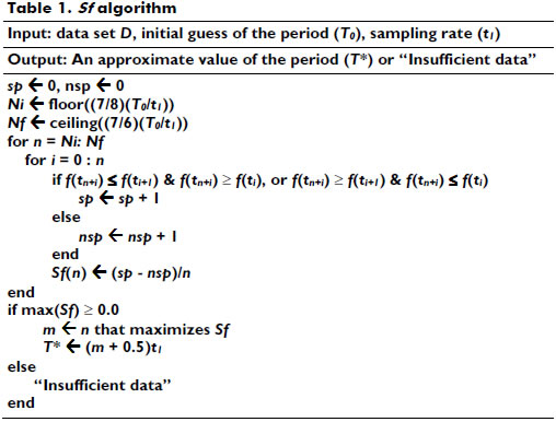
The error Sf(n) corresponds to a measure of the periodicity of the values between two consecutive sections for a candidate period value t of the target function. The functional Sf(n) remains piecewise constant on the interval [t_i,t_i+1). Therefore, any approximation of T on the basis of D cannot be guaranteed to be any closer than half of the radius of the partition, t₁/2, to T. The algorithm returns a value of T* = (m + 0.5)t₁ such that m maximizes Sf(n) over the interval [tNi,tNf].

If the comparison between two sections results in zero points being shuffled, then Sf = -1. In contrast, if all the points are shuffled, Sf = 1. The bound Sf = 0.0 may be used as a threshold to guarantee the quality of the approximation. This threshold implies that the number of shuffling points should be at least equal the number of non-shuffling points to guarantee the quality of the approximation. If the output of the algorithm Sf is insufficient data, then t₁ should be changed before running the algorithm again.

2) Second algorithm: Δf

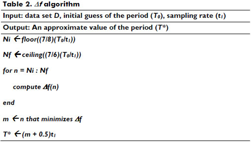
N will denote the unique (unknown) n such that tN ≤ T < t_N+1. With this notation in place, we now turn to the description of the algorithm for estimating T. The second algorithm, Δf(n), minimizes the error functional written in Equation (1) over the sampling partition of the interval [tNi, tNf] into intervals of the same length t₁, as defined in Table II.

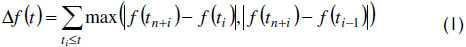
The functional Δf in Table 2 measures the difference between data points for two sections. Thus, the best candidate period exhibits the smallest difference between sections.

Illustrative example

Consider the target signal f(t) = (1/2π)sin(5t)t, which belongs to the third group of functions ("hard" functions) and which is chunked with period T = 2π, where N = 100 and DN = 0.5. Figure 3 shows that the maximum Sf matches the true period. Notice that every candidate period different from the best candidate results in negative measurements of the functional Sf. In addition, the maximum Sf surpasses zero, which was defined as the quality threshold for the approximation.

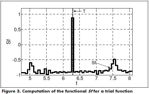
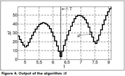
Given a maximum possible error in the first approximation (T0) equal to 14.2%, and limits [tNi tNf] equal to [7T₀/8 7T₀/6], Figure 3 and Figure 4 show the total search range, which consequently covers [3T/4 4T/3]. In addition, Figure 4 shows the situation using the functional Δf. The exploration of the search range shows two local minima, which justifies the search for the global minimum.

Quality of the approximation

This section presents the results of two experimental evaluations used to analyze the quality of the approximations given by Δf and Sf. The first evaluation analyzes the performance of both algorithms using noiseless data, whereas the second evaluation studies the influence of noisy data on the quality of the estimations.

The evaluation of the algorithms for noiseless data focuses on the relative error, defined as Er = |T - T*| / t₁, for Δf and Sf under a wide range of sampling periods as well as for the 25 functions from the three groups: friendly, tractable, and hard. This analysis is comprised of three steps: 1) setting the value of the true period T (for instance, to 2p); 2) defining a sampling period as well as a function for each experiment to generate artificial data; and, finally, 3) computing both approximations. Now, given that the sampling period depends on N and ΔN according to t₁ = T / (N - 1 + ΔN), this analysis uses 64 ≤ N ≤ 190 and 0 ≤ ΔN < 1, as shown in Figure 5.

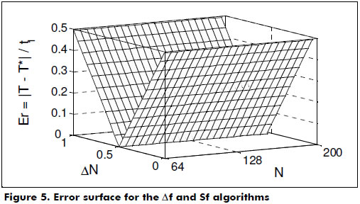
The errors for both estimations in Figure 5 proved to be equal because both approximations have the same value in every experiment. We compare this result with the error surface for a periodogram estimation in Figure 1. The "V" shape for the error shows that the approximations do not depend on the number of data points per period, N, or on the harmonic content. The approximations depend only on the value of ΔN; thus, a constant average value in the signal (null frequency) does not have any influence on the approximation. In addition, Er has a bound equal to 0.5, which guarantees approximations for noiseless data under half of a sampling period.

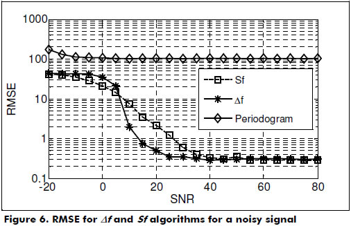
A second experimental evaluation to measure the quality of the approximations focuses on the performance of the algorithms under noisy conditions. Traditionally, the Signal-to-Noise-Ratio (SNR) measures the noise content of a signal. Thus, for each SNR, given in decibels, the analysis required 1×10⁵ Monte Carlo simulations. Each experiment results in a relative error (Er = |T - T*| / t₁), and the set of all 1×10⁵ results per SNR generates an error equal to their mean squared error (RMSE).

Each Monte Carlo simulation randomly changes several parameters to evaluate the influence of those parameters on the performance of an algorithm. In this case, the parameters N, ΔN, and T₀ vary between the bounds 70 ≤ N ≤ 300, 0 ≤ ΔN < 1, and 3/4T ≤ T₀ ≤ 5/4T, respectively. In addition, for each trial, the Monte Carlo method chooses a function from among the six trial functions used in this paper. Finally, the true period randomly varies over 10 possible values: 3/2, 3/4 1/2, 4/5, 1, π, √2, e¹, (1+√5)/2, √3.

High SNRs (higher than 40 dB in Figure 6) have an asymptote corresponding to the average of the "V" shape in Figure 5, which equals 0.25. In addition, Figure 6 also shows that the Δf algorithm performs better than does the Sf algorithm for SNRs from 5 to 40 dB, which is a normal noise content for a signal such as the data collected for the tracking frequency in the next section. This difference in the range of 5-40 dB can be explained by properties of the algorithms. Remember that Sf discretizes the contribution of each data point, adding one or zero to Sfi, whereas Δf uses the difference between two data points to define Δf_i. Both algorithms, however, exhibit the same performance for noiseless or quasi-noiseless data points. Figure 6 also shows a poor performance for the periodogram, which is mainly caused by the "hard" functions (two of the six trial functions) because they do not meet the restrictions of a periodogram.

Applications

This section shows the application of the proposed algorithms for the estimation of the period in two classical problems. The first part approximates the period of a Van der Pol oscillator, and the second part approximates the power grid frequency.

Van der Pol oscillator

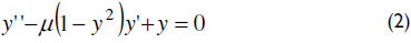
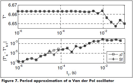
A Van der Pol oscillator is a nonlinear dynamical system. The mathematical model for this oscillator corresponds to the differential equation in equation (2). The application in this paper uses a computer to find the solution of the system when μ = 1, with initial conditions y(0) = 2, y´(0) = 0.

The approximation of the period starts with a coarse estimation, for instance, T₀ = 6.6 s, and a sampling period, t₁, equal to 0.1 s. Then, the Δf and Sf algorithms produce the first approximations T* = 6.65. These approximations serve as initial guesses (T₀) for the second iteration, which differs from the initial iteration by a reduced sampling period, as show in Figure 7. In summary, this iterative process uses an approximation at the end of an iteration as an initial guess for the subsequent iteration but using a reduced sampling period for each run. The absolute value of the difference between approximations at consecutive iterations, as shown in the lower part of Figure 7, demonstrates the convergence of the method. The best estimation in Figure 7 uses a sampling period t₁ = 1×10-6 s, which results in an approximated period of T* = 6.663250 s.

Power grid frequency

Most of the algorithms used for estimating the power grid frequency assume a perfect sinusoidal wave as a base for their estimations. For example, the algorithm proposed in the IEEE standard 1057TM-2007 for Digitizing Waveform Recorders (IEEE Standard, 2011) minimizes the square error between a sinusoidal wave and the data. The IEEE standard 1057TM-2007 presents an iterative method for approximating the amplitude, phase, continuous component and frequency of a sinusoidal signal. This method accurately approximates a frequency for signals with low harmonic content, but the estimation degrades as the signal deviates from a perfect sine wave. Other algorithms base their results on the Discrete Fourier Transform, Kalman Filters, and maximum likelihood estimates, among many other techniques.

The application of the Δf algorithm in this section implies a reduction from a nominal voltage (120 V) to 5 V using a transformer. This reduction allows a data acquisition card (NI 6024E) and Matlab to record data at a maximum sampling rate of 5 μs, which corresponds to 3333 data points per period at the nominal frequency (60 Hz). The analysis of the quality of the estimations uses the measurements from a three-phase power quality and energy analyzer, the Fluke 435, as a reference.

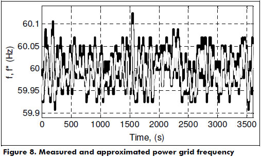
Limitations of the analyzer set the interval between approximations to half a second. Thus, every 500 ms, Matlab records data in real time for 50 ms, and subsequently, the Δf algorithm generates a candidate period using a constant T0 = 1/60 s. The maximum sampling rate of the data acquisition card (5 μs) limits the precision to 0.01 Hz, while the precision of the analyzer exceeds this precision by ten times. However, remember that the error in the Δf approximation equals half of t₁ for noiseless data. Thus, the precision of Δf may be increased by simply using a faster acquisition card. This experiment was carried out in October 22 of 2013, from 12:49 through 13:49 in Bogotá, Colombia.

Figure 8 shows the estimations given by the Δf algorithm (black line) and by the analyzer (white line). The figure shows that the estimation algorithm Δf properly tracks the power grid frequency.

Conclusions

The value of an estimated period highly influences a number of processes, such as signal reconstruction; for instance, errors of less than 5% in the period may cause errors exceeding 50% in the approximation of some harmonics. One of the most common techniques used to estimate periods, a periodogram, as well as other algorithms assume a certain sampling rate or may also require prior knowledge about the signal, such as the function shape, rendering them useless in many practical applications. In contrast, this paper presents two algorithms, Δf and Sf, that guarantee a bounded relative error equal to half of the sampling rate, additionally assuring complete independence between the harmonic content for noiseless data and the estimations. The results for noisy signals also proved promising. In addition, future studies may seek to reduce the amount of data required to obtain an approximation, for instance, only using a representative subset of the data to generate a candidate period instead of using the whole data set.

References

Bernieri, A., Ferrigno, L., Laracca, M., & Landi, C. (2010). Efficiency of active electrical power consumption in the presence of harmonic pollution: a sensitive analysis. Paper presented at the Instrumentation and Measurement Technology Conference (I2MTC). http://dx.doi.org/10.1109/IMTC.2010.5487994        [ Links ]

Bernieri, A., Betta, G., Ferrigno, L., & Laracca, M. (2012, May). Electrical energy metering in compliance with recent european standards. Instrumentation and Measurement Technology Conference (I2MTC). http://dx.doi.org/10.1109/I2MTC.2012.6229455        [ Links ]

Candan, C. (2011). A method for fine resolution frequency estimation from three DFT samples. IEEE Signal Processing Letters, 18(6), 351-354. http://dx.doi.org/10.1109/LSP.2011.2136378        [ Links ]

Chudamani, R., Vasudevan, K., & Ramalingam, C. S. (2009). Real-time estimation of power system frequency using nonlinear least squares. IEEE Transactions on Power Delivery, 24(3), 1021-1028. http://dx.doi.org/10.1109/TPWRD.2009.2021047        [ Links ]

IEEE Std. 1057TM-2007 (2007). IEEE Standard for Digitizing Waveform Recorders. NJ, USA: Institute of Electrical and Electronic Engineers.         [ Links ]

McKilliam, R. G., Quinn, B. G., Clarkson, I. V. L., & Moran, B. (2010). Frequency estimation by phase unwrapping. IEEE Transactions on Signal Processing, 58(6), 2953-2963. http://dx.doi.org/10.1109/TSP.2010.2045786        [ Links ]

Pantazis, Y., Rosec, O., & Stylianou Y. (2010). Iterative estimation of sinusoidal signal parameters. IEEE Signal Processing Letters, 17(5), 461-464. http://dx.doi.org/10.1109/LSP.2010.2043153        [ Links ]

Petrovic, P. B., & Stevanovic, M. R. (2011). Algorithm for Fourier coefficient estimation. IET Signal Process, 5(2), 138-149. http://dx.doi.org/10.1049/iet-spr.2009.016        [ Links ]

Provencher, S. (2010). Estimation of complex single-tone parameters in the DFT domain. IEEE Transactions on Signal Processing, 58(7), 3879-3883. http://dx.doi.org/10.1109/TSP.2010.2046693        [ Links ]

Stoica, P., & Moses, R. (2005). Spectral Analysis of Signals. New Jersey: Prentice Hall Inc.         [ Links ]

So, H. C., Chan, F. K. W., & Weize, S. (2011). Subspace approach for fast and accurate single-tone frequency estimation. IEEE Transactions on Signal Processing, 59(2), 827-831. http://dx.doi.org/10.1109/TSP.2010.2090875        [ Links ]

Ta-Hsin, L., & Kai-Sheng, S. (2009). Estimation of parameters of sinusoidal signals in non-Gaussian Noise. IEEE transactions on Signal Processing, 51(1), 62-72. http://dx.doi.org/10.1109/TSP.2008.2007346        [ Links ]

Ta-Hsin, L. (2013). Times Series with mixed spectra. Boca Raton: Chapman and Hall Book, CRC Press.         [ Links ]

Yang, C., & Wei, G. (2011). A noniterative frequency estimator with rational combination of three spectrum lines. IEEE Transactions on Signal Processing, 59(10), 5065-5070. http://dx.doi.org/10.1109/TSP.2011.2160257        [ Links ]