DOI: http://dx.doi.org/10.15446/ing.investig.v35n2.47763.

Kinematics modeling and simulation of an autonomous omni-directional mobile robot

Modelado y simulación de un robot móvil autónomo omni-direccional

D. Garcia-Sillas¹, E. Gorrostieta-Hurtado², J. E. Vargas³, J. Rodríguez-Reséndiz⁴, and S. Tovar⁵

¹ Daniel García Sillas. Electronical Engineer, Instituto Tecnológico de Querétaro, México. Master in Distributed Software Engineering, Universidad Autónoma de Querétaro, México. Affiliation: Member of IEEE, México. E-mail: dgarcia37@alumnos.uaq.mx.
² Efrén Gorrostieta Hurtado. Dr. Eng. Mechatronics, Centro de Ingeniería y Desarrollo Industrial, México. Affiliation: Senior Member IEEE, México. E-mail: efrengorrostieta@gmail.com.
³ J. Emilio Vargas Soto. Dr. in Physics Science, Universidad Complutense de Madrid, Spain. Post Doctorade by The Electrocommunication University of Tokyo, Japan. Affiliation: Senior Member IEEE, México. E-mail: emilio@mecatronica.net.
⁴ Juvenal Rodríguez Reséndiz. Dr. in Engineering, Universidad Autónoma de Querétaro, México. Affiliation: Senior Member IEEE, México. E-mail: juvenal@uaq.edu.mx.
⁵ Saúl Tovar Arriaga. Dr. in Biomedical Sciences, Friedrich Alexander University Erlangen, Germany. Affiliation: Senior Member IEEE, México. E-mail: saul.tovar@uaq.mx.

How to cite: Garcia-Sillas, D., Gorrostieta-Hurtado, E., Vargas, J. E., Rodríguez-Reséndiz, J., & Tovar, S. (2015). Kinematics modeling and simulation of an autonomous omni-directional mobile robot. Ingeniería e Investigation, 35(2), 74-79. DOI: http://dx.doi.org/10.15446/ing.investig.v35n2.47763.

ABSTRACT

Although robotics has progressed to the extent that it has become relatively accessible with low-cost projects, there is still a need to create models that accurately represent the physical behavior of a robot. Creating a completely virtual platform allows us to test behavior algorithms such as those implemented using artificial intelligence, and additionally, it enables us to find potential problems in the physical design of the robot. The present work describes a methodology for the construction of a kinematic model and a simulation of the autonomous robot, specifically of an omni-directional wheeled robot. This paper presents the kinematic model development and its implementation using several tools. The result is a model that follows the kinematics of a triangular omni-directional mobile wheeled robot, which is then tested by using a 3D model imported from 3D Studio^® and Matlab^® for the simulation. The environment used for the experiment is very close to the real environment and reflects the kinematic characteristics of the robot.

Keywords: Mobile robots, robotics, kinematics, modeling and simulation.

RESUMEN

Aunque la robótica ha avanzado hasta el punto de ser relativamente accesible con proyectos de bajo costo, aún cabe la necesidad de crear modelos que representen fielmente el comportamiento físico de un robot creando una plataforma completamente virtual. Esto nos permite, por un lado, probar algoritmos de comportamiento o de inteligencia artificial y, por otro lado, encontrar probables problemas en el diseño físico. El presente trabajo propone el modelado cinemático y la simulación de un robot móvil autónomo, particularmente de un robot omni-direccional con ruedas. Se plantea la metodología para la construcción del modelo cinemático así como su implementación utilizando diversas herramientas. El resultado es un modelo que representa a un robot móvil omni-direccional triangular con ruedas, que fue probado utilizando un modelo tridimensional importado de 3D Studio^®, y utilizando Matlab^® para la simulación del modelo. También se implementa el mismo modelo utilizando una herramienta dedicada a la simulación de robots, que ofrece un ambiente muy completo de simulación. El ambiente de simulación ofrece un comportamiento muy cercano al real y refleja las características cinemáticas del robot.

Palabras clave: Robots móviles, robótica, cinemática, modelación y simulación.

Received: December 9th 2014 Accepted: March 20th 2015

Introduction

Nowadays, there is a fast-growing interest in robotics and mechatronics systems, since robotics platforms performing different tasks are increasingly common in daily life. They can be seen in industry where it is common for them carry out tasks such as welding, painting, stacking (manipulators) and other processes like transporting or conveying objects from one place to another. Mobile robots can be legged or wheeled, or even a combination of both, depending on the kind of application for which they are intended to be used. Mobile robots can adopt a large variety of forms, sizes, and types of mobility which allow them to function in their environment whether it be land, air or water; they can be flying devices or they could even be submarine or amphibious (Rui Ding et al., 2009). Some of these morphologies are inspired by the animal kingdom, where fish or dolphin-like swimming movements can be integrated (Yu, J., et al., 2012) showing a very natural gait.

Autonomous systems are gradually part of our way of life, regardless of notice it or not. The increased use of intelligent robotic systems in indoor or outdoor applications demonstrates the efforts made by researchers in many places. Autonomous systems have greater autonomy than before, and often new applications emerge, ranging from transport systems in industrial plants, transport systems at airports, for rescue systems, and even in health and care institutions.

Another important point to mention is that although autonomous robotic systems include their own set of sensors, actuators and computers there is a possibility that they are controlled from open systems in networks with distributed control systems.

This causes to emerge new and more daring applications for mobile robots. For example, one of the most important trends of the past decades has been the increased use of mobile robots on rough terrain such as mines, forests, areas of disasters and planetary surfaces, since some of these surfaces may be inaccessible to human or perhaps dangerous. To meet the requirements of these trends a greater degree of complexity to mobile robots needs to be implemented, since they need to deal with changing environments by employing a wider variety of resources like sensors sets, actuator and decision making algorithms. This does not happen for other types of robots such as manipulators or stationary robotic platforms since fewer requirements are needed to operate.

Mobile robots have much more freedom and are more flexible than manipulators, but this implies that modelling them results in more complicated models than those for manipulators.

From the viewpoint of kinematics, the main difference between a manipulator and a mobile robot is the nature and disposition of its joints (Li Xiang, et al., 2008). The manipulator robot is usually modeled as an open kinematic chain composed of an alternation of rigid bodies with joint elements of a single degree of freedom. By contrast, the kinematic structure of a mobile robot can be considered as a set of closed kinematic chains, as much as wheels in contact with the ground. Furthermore, the wheel-ground interaction is defined, from the kinematic point of view, as a planar joint with three degrees of freedom, where one of them, usually uncontrolled, represents lateral slippage. These two facts make the construction of the model more difficult.

In the following section of this paper a methodology to obtain a kinematic model of an omni-directional wheeled vehicle based on the jacobean matrix is proposed. After that, the model is tested by executing a simulation using the obtained model by using a couple of software tools. The approach proposed in this paper employs a different simulation environment already proposed (Muñoz, 2010); it resides in the simulation platform that was built in a 3D system where objects can be added to the scene, which in turn gives a more realistic feeling. Additionally, the development was concluded with the construction of the physical model in order to start working in areas like motion and tracking control. Some results are shown in the penultimate section. Further developments and conclusions are discussed in the final section of this document.

Kinematics

The robot's motion study is based accordingly to its geometry and considering the following constraints:

• The robot is moving over a flat surface.

• There are no flexible components in the robot's structure.

• Friction is not take into consideration

Wheels behave as a planar joint of DoF as described below.

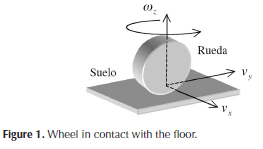
Assuming that the wheel is a rigid element, it is always in contact with the ground in a single point and it serves as the origin for the references system shown in Figure 1. Direction v determines the normal direction of the wheel, v represents the side's slippage and w_z is the rotational speed when the robot turns. In the case of a conventional wheel the component v_x is null, but there are other wheels providing a different behavior as shown in Figure 2.

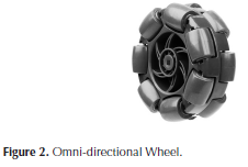
The omni-directional wheel is defined as a standard wheel provided by a rollers array, whose axis turn perpendicularly to the normal wheel direction (Jae-Bok Song, et al., 2008). In this way, when force is applied to its side, component v_x is no longer null.

The robot has multiple legs with three degrees of freedom (DoF) each, which gives it the capability to execute dexterous movements. Particularly, this robot has three legs, and each one of them has three DoF and they all are bidirectional.

The floor coordinate system {M} is fixed relative to the surface and it stands for the coordinate reference system for the robot motion.

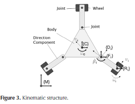
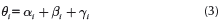
The corresponding global position of the robot is represented by {C}, which is associated to the robot body; its cartesian position is given by X_c, Y_c, and its angle by θ_c.

{F_i} is the i-th leg joint attached to the robot body. The angle α_i represents the orientation relative to {C}, and λ_i describes its position vector.

{D_iJ refers to the directional component of the i-th wheel.

The directional angle is represented by β_i.

{R_i} represents the systems located at the contact point with the floor of the i-th wheel. The angle and position vector between the current and the previous systems are γ_i and δ_i respectively.

The linear speed of the robot is given by the Equation 1 (Muñoz, 2010):

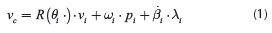
Where R(θ_i) represents the rotation matrix on the plane; ρ_i and θ_i are defined as the position and orientation vector or the systems {R_i} seen from {C}, indicated as follows:

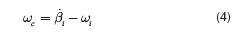
The robot angular speed is calculated by:

The mentioned equations above are arranged as a jacobean matrix such that:

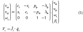
Whereand v_cx are the components belonging to v_cy, ρ_jx and ρ_iy to ρ_i, λ_ix and λ_iy to λ_i, and finally v_ix and v_iy to v_i , respectively. Additionally, c_i and s_i represent the cosine and sine of the angle θ_i.

The linear speed of the wheels is obtained from the applied action of a motor. In the case of a conventional wheel, with traction but non-directional, with a radius r_i and a rotation speed W_ix, a matrix can be defined as follows:

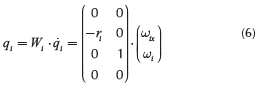
Equation 6 allows to introduce the angular speed w_ix and to override the directional action of β_i. If the wheel can have direction, matrix W_i will be represented as follows:

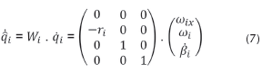
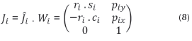
The jacobean matrix of the i-th wheel represented by j_i with or without direction is defined as the model that allows to compute the robot's speed V_c according to the vector components q_i .For example, in case of a non-directional wheel, Equations (5) and (6) are combined as follows:

Considering n wheels attached to the robot and according to Equation 5, a set of equation systems is proposed, where the speeds vector V_c must satisfy simultaneously the following constraint (Calandín, 2006):

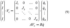
where the matrix l represents the identity matrix.

Next, least squares approach is used to find a solution for the vector V_c :

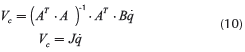
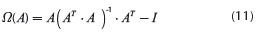
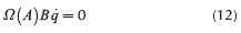
Matrix J then represents the whole jacobean system of the robot. Equation (11) states that the robot has a no-slip condition assuming that the robot is correctly actuated:

And it can be expressed as follows:

Methodology

Figure 4 shows the robot kinematic setup, and it represents a particular geometric configuration of an omni-directional vehicle that is being pursued in this study. It defines an equilateral triangle with a wheel installed on each one of its vertexes.

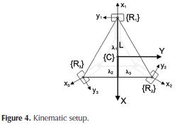
The distance from the origin {C} is its own geometrical center to any of the wheels in question here given by L. All wheels are directional and therefore they can be translated as an equality {F_c} = {D_c} = {R_c}, it means for every i, β_i= 0° y y_i= 0°

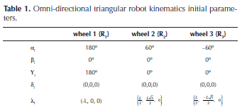
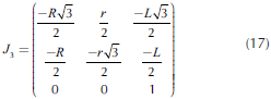
Table 1 comprises the initial parameters for the kinematic model. In order to obtain the jacobean for every wheel, matrix J_i given in (5) is multiplied by the wheel conversion matrix of the actuated wheel for an omni-directional shown in (13):

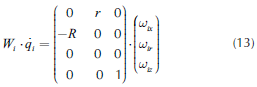
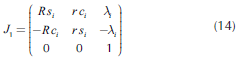
Matrix W. models a radius R wheel, omni-directional with radius r and rollers fixed to 90°, with traction but non-directional. Regarding vector q, W_ix represents the angular speed of the motor attached to the wheel, W_ir is the wheel's rollers angular speed and W_iz holds the rotational slippage in relation to the vertical axis of the wheel. Then, the jacobean for the i-th wheel can be expressed as follows:

Substituting the parameters in table 1 in Equation 14, a jacobean for each wheel is obtained:

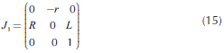
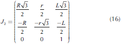
Matrixes J₁, J₂and J₃ are combined in Equation (9) and the entire vehicle jacobean is solved as described in (10):

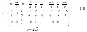
Matrix in (18) contains the relation between the vehicle speed and the rollers, but from a practical point of view only actuated degrees are taken, such that the non-slippage condition is used by applying Equation (11):

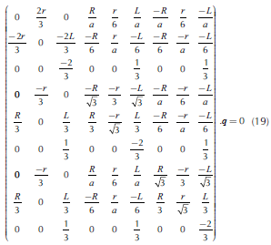
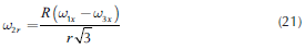
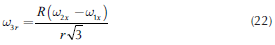
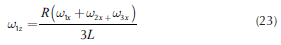
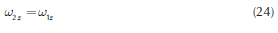
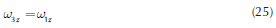
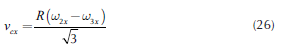
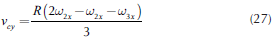
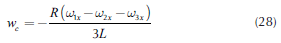
This matrix in (19) results indeterminate since there are three rows that are linear combination from the others. Because of this condition, non-actuated variables are removed accordingly to the actuated, and the following equations are obtained:

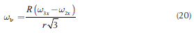
By substituting all equations obtained in equation (18), the global speed of the wheels can be calculated:

Equations can be accommodated as a matrix and the final Jacobean of the robot is obtained:

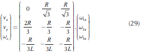
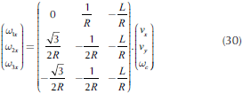
The inverse of the Jacobean (29) of the robot can be expressed as follows:

Simulation

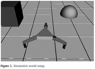
A simulation environment was setup in order to run the model and test the kinematic model. A 3D-model world was built using 3D Studio^® where all the mechanical parts of the robot are represented within the scheme. Later on, 3D world created in 3D Studio^® is loaded into MatLab^® (Figure 5), where the kinematic model is programmed and computed to simulate the robot motion.

The studied model is a holonomic system that allows omni-directional motion and, therefore, any angular and linear speed combination as well. These conditions let the robot make any possible move on a plane surface.

To test the model, a basic configuration on the wheel speed was programmed to generate different moves.

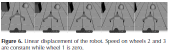
Linear movement

This type of movement is defined by a linear speed described by the components v_cx and v_cy. These components must be constant to let the robot move iinearly and the angular speed θ_c null. Figure 6 shows the linear speed of the robot:

Rotational movement

In this case, the robot is spinning on its center. Components v_cx and v_cy are null, while θ_c remains constant (Figure 7).

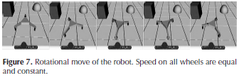
As seen in the figures above, the robot can lead to any path based on the speed of the wheels; varying such speeds the direction of the robot can change making it go to any other place on a flat plane.

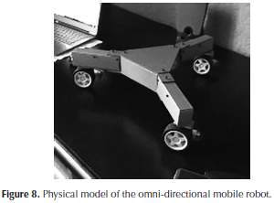
Following the interest on the robotic platform proposed here, a physical model has been built (Figure 8). The robot is provided with nine DoF. It has three legs as described in the present article, and each one of them has two motors controlling its position, and a bi-directional DC motor providing mobility to the robot. The legs position and motor speed are controlled by an Arduino development kit.

Conclusions

In the present paper a kinematic model of an omni-directional mobile robot and its simulation have been conducted. Forward and inverse kinematic models have been proposed.

The paper has two main parts: in the first section, the calculation of the kinematic models required by any controller to compute the current position of the robot is presented. Forward and inverse models needed to compute position based on the speed of the wheels and speeds needed to achieve certain position respectively are shown; in the second part, a simulation was developed in order to demonstrate full functionality of the kinematic modelling for the robot, where the results presented are very satisfactory. Two basic motion tests were performed and they were intended to demonstrate the feasibility of the model.

There is great interest in applying the models of the robot in a specific job in the future. One of the intentions of developing simulator robots or even physical construction is to use them to develop algorithms that can automatically control certain required behavior (Cárdenas, et al., 2011). Computer software like MatLab^® is one of the tools used where artificial intelligence is needed to manipulate the robot without spending much developing time. Trajectory generation and control of mobile robots with artificial intelligence could be implemented using these techniques (Nardenio A. Martis, et al., 2008).

References

Calandín, L.I.G. (2006). Modelado cinemático y control de robots móviles con ruedas (Doctoral dissertation, Universitat Politècnica de València).         [ Links ]

Cárdenas, E.F., Mendez, L.M., & Esmeral, J.S. (2011). Métodos para generar trayectorias libres de colisiones en entornos multidimensionale. Ingeniería e Investigación, 31(2), 5-17.         [ Links ]

Jae-Bok Song, & Kyoung-Seok Byun. (2008). Design and Control of an Omnidirectional Mobile Robot with Steerable Omnidirectional Wheels. Korea University, Mokpo National University. Republic of Korea. P223.         [ Links ]

Martins, N.A., Bertol, D., Lombardi, W.C., Pieri, E.R., & Dias, M.M. (2008, October). Neural control applied to the problem of trajectory tracking of mobile robots with uncertainties. In Neural Networks, 2008. SBRN'08. 10th Brazilian Symposium on (pp. 117-122). IEEE. DOI: 10.1109/sbrn.2008.41.         [ Links ]

Xiang, L., Xunbo, L., & Liang, C. (2007, December). Multi-disciplinary modeling and collaborative simulation of multi-robot systems based on HLA. In Robotics and Biomimetics, 2007. ROBIO 2007. IEEE International Conference on (pp. 553-558). IEEE. DOI: 10.1109/robio.2007.4522222.         [ Links ]

Rui Ding, Junzhi Yu, Qinghai Yang, & Min Tan. (2009). Kinematics Modeling and Simulation for an Amphibious Robot: Design and Implementation. Institute of Automation, Chinese Academy of Sciences. Beijing 100190, China.         [ Links ]

Yu, J., Ding, R., Yang, Q., Tan, M., Wang, W., & Zhang, J. (2012). On a bio-inspired amphibious robot capable of multimodal motion. Mechatronics, IEEE/ASME Transactions on, 17(5), 847-856. DOI: 10.1109/TMECH.201 1.2132732.         [ Links ]

Muñoz M.V.F., Gil-Gómez, G., & García, C.A. (2003). Modelado Cinemático y Dinámico de un Robot Móvil Omni-Direccional. Universidad de Málaga. Parque Tecnológico de Andalucía C/Severo Ochoa 4, 20590 Málaga.         [ Links ]