


Serviços Personalizados
Journal
Artigo
 Inglês (pdf)
 Artigo em XML
 Referências do artigo
 Enviar este artigo por email
Indicadores
-
 Citado por SciELO
 -
 Acessos
Links relacionados
-
 Citado por Google
 -
 Similares em
SciELO
Similares em
SciELO -
 Similares em Google
Compartilhar

 Permalink
Ingeniería e Investigación
versão impressa ISSN 0120-5609
Ing. Investig. vol.35 no.3 Bogotá set./dez. 2015
https://doi.org/10.15446/ing.investig.v35n3.49391
DOI: http://dx.doi.org/10.15446/ing.investig.v35n3.49391.
A recursive formula for the evaluation of earth return impedance on buried cables
Una fórmula recursiva para la evaluación de la impedancia de retorno por tierra en cables subterráneos
R. Iracheta-Cortez1
1 R. Iracheta Cortez: PhD in Electrical Engineering, CINVESTAV Guadalajara, Mexico. Affiliation: Postdoctoral Fellow at Centro de Investigación en Matemáticas, A.C., CIMAT. Guanajuato, Mexico.
E-mail: reynaldo.iracheta@cimat.mx.
How to cite: Iracheta-Cortez, R. (2015). A recursive formula for the evaluation of earth return impedance on buried cables. Ingeniería e Investigación, 35(3), 34-43. DOI: http://dx.doi.org/10.15446/ing.investig.v35n3.49391.
ABSTRACT
This paper presents an alternative solution based on infinite series for the accurate and efficient evaluation of cable earth return impedances. This method uses Wedepohl and Wilcox's transformation to decompose Pollaczek's integral in a set of Bessel functions and a definite integral. The main feature of Bessel functions is that they are easy to compute in modern mathematical software tools such as Matlab. The main contributions of this paper are the approximation of the definite integral by an infinite series, since it does not have analytical solution; and its numerical solution by means of a recursive formula. The accuracy and efficiency of this recursive formula is compared against the numerical integration method for a broad range of frequencies and cable configurations. Finally, the proposed method is used as a subroutine for cable parameter calculation in the inverse Numerical Laplace Transform (NLT) to obtain accurate transient responses in the time domain.
Keywords: Earth-return impedance, Pollaczek's integral, Wedepohl's integral, infinite series expansion, recursive formula, buried cables, Numerical Laplace Transform (NLT).
RESUMEN
En este artículo se presenta una solución alternativa basada en series infinitas para la evaluación precisa y eficiente de la impedancia de retorno por tierra en cables subterráneos. En este método se utiliza la transformación de Wedepohl y Wilcox para descomponer la integral impropia de Pollaczek en un conjunto de funciones de Bessel más una integral definida. La característica principal de las funciones de Bessel es que son fáciles de calcular con herramientas modernas de software matemático como Matlab. Las principales contribuciones de este artículo son la aproximación de la integral definida por una serie infinita, dado que no tiene solución analítica, y su evaluación numérica por medio de una fórmula recursiva. La precisión y eficiencia de la fórmula recursiva se compara contra el método de integración numérica para un amplio rango de frecuencias y configuraciones de cables subterráneos. Finalmente, se utiliza el método propuesto como una subrutina de cálculo de parámetros de cables en la Transformada Numérica de Laplace (NLT) para obtener respuestas transitorias precisas en el dominio del tiempo.
Palabras clave: Impedancia de retorno por tierra, Integral de Pollaczek, Integral de Wedepohl, serie infinita, fórmula recursiva, cables subterráneos, Transformada Numérica de Laplace (NLT).
Received: February 27th 2015 Accepted: July 22nd 2015
Introduction
The accurate evaluation of the frequency-dependent earth return impedance is extremely important to perform reliable studies of electromagnetic transient on transmission lines and cables as well as to carry out analysis of electromagnetic interference. The most widely known and accepted expressions for the evaluation of this parameter were first published by Carson (1926), for being used with aerial lines, and then by Pollaczek (1926), for their use with buried cables and combinations of buried cables and overhead conductors. These expressions are given by a set of improper integrals that do not have an analytic closed form solution. Traditionally, numerical integration methods and approximate formulas have been widely discussed in the specialized literature to solve these improper integrals (Ametani, 1980; Deri et al., 1981; Dubanton et al, 1969; Legrand et al., 2008; Nguyen, 1998; Papagiannis et al., 2005; Saad et al., 1996; Uribe et al., 2004 and Zou et al., 2011). It has been demonstrated that both approaches can be implemented successfully for solving Carson's integral, whose integrand behavior is non-oscillatory. Nevertheless, due to the fact that Pollaczek's integral is highly oscillatory, its solution with direct numerical integration methods in a conventional PC is very time-consuming. Moreover, approximate formulas published in the literature for buried cables are only valid for certain frequency ranges and cable configurations.
Apart from the aforementioned facts, the contribution of the earth-return impedance on buried cables is much more significant than in aerial lines. First, the self and mutual earth return impedance constitutes more than two thirds of the series impedance matrix on buried cables. Second, the frequency-dependent earth-return impedance has to be evaluated at many discrete points to obtain a good resolution of the transient response in the time domain. It is therefore crucial to develop efficient and accurate tools for the evaluation of earth return impedances on buried cables.
In 1973, Wedepohl and Wilcox published an exhaustive analysis of Pollaczek's integral, which has been largely ignored (Wedepohl and Wilcox, 1973). The main contribution of these authors has been the decomposition of Pollaczek's integral in a set of improper integrals plus a definite integral. The improper integrals are approximated with Bessel functions, which are easy to compute in modern mathematical tools such as Matlab. These authors also derived an infinite series solution to the definite integral. To date, the main problem with such series solution is that it has been cumbersome to implement.
Uribe and Ramirez have made some efforts to implement this series solution for a limited frequency range (Uribe and Ramírez, 2012). On the other hand, Theodoulidis (2012) has proposed the use of special functions such as 'hypegeometric' in Matlab to approximate the definite integral. However, the computation of built-in hypergeometric function in Matlab is generally slow, and this routine is also susceptible to failure for cases of extreme parameters. Thus, this paper uses Wedepohl and Wilcox's decomposition for solving the definite integral with an alternative solution based on infinite series. The numerical implementation of this approach is done through a recursive formula that can be applicable for a broad range of frequencies and cable configurations.
Earth return impedance on buried cables
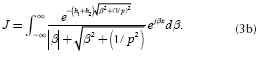
In 1926, Pollaczek published a set of improper integrals to evaluate the electromagnetic coupling caused by an infinite thin filament in the presence of an imperfect conducting soil (Pollaczek, 1926; Dommel, 1986). The general expression derived by Pollaczek to evaluate the mutual impedance between two buried cables is given by:
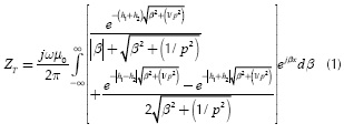
Where ω is the angular frequency in rad/s, µ0 ( µ0 = 4π x10-7 Wb/(A·m)) is the magnetic permeability of free space, β is the dummy variable, x is the horizontal distance between cables, h1 and h2 are the depths of cables 1 and 2 and  is the complex depth with the ground resistivity ρsoil. This earth model assumes that µ0 = µground and the soil is a homogeneous medium whose flat surface divides the space into two semi-infinite regions: soil and air. The second term in Equation (1a) can be simplified by
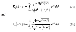
where K0 is the modified Bessel function of second type and order zero. By replacing Equation (2a) and Equation (2b) in Equation (1a), ZT becomes:
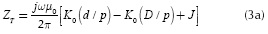
where
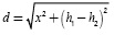 is the distance between cables,
 is the complex depth, and
 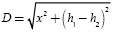 is the distance between a real cable and the image from the other one. Physical variables h1, h2, x, D and d and their geometric relationships are depicted in Figure 1. The remaining term J is Pollaczek's integral.
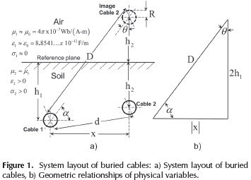
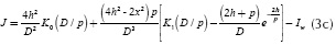
It should also be noted that Equations (3a) and (3b) become the self-earth return impedance when x is the conductor radius R and h1= h2.
In 1973, Wedepohl and Wilcox introduced the following analytical decomposition for (3b):
Where
and where h = (h1+h2) / 2 and t = 2h/D.
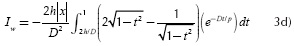
The modified Bessel functions K0 and K1 in (3c) evaluate improper integrals via convergent series. These special functions become easy to compute in modern mathematical tools such as Matlab. The second term in Equation (3c) has an algebraic expression that does not present computational difficulties. The third term Iw in (3c) is named in this paper as the Wedepohl-Wilcox's integral. This definite integral does not have an analytical solution, but can be easily computed with any numerical integration methods. Wedepohl and Wilcox (1973) have proposed an infinite series solution for Iw that to date is still awkward to implement for a broad range of frequency ranges and cable configurations. Later these authors also proposed an approximate formula for calculating the earth return impedance ZT on buried cables. However, its range of application is limited for low frequency or a factor |D /p| ≤ 1/4.
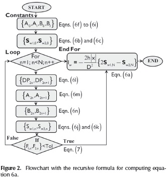
Series solution and recursive formula
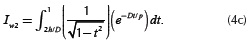
A recursive formula is developed from the Wedepohl-Wilcox's integral (Iw). For the analysis, let (3d) as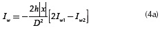
Where
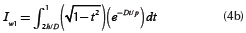
and
The exponential term of these equations is replaced by
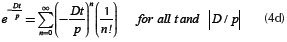
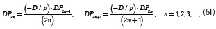
which is absolutely convergent for all t and |D / p|. The dimensionless variable t is limited to 0 < t < 1. Thus, the infinite series solution for (4b) and (4c) is
and
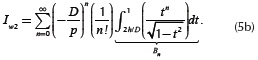
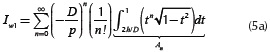
These infinite series can be solved via a recursive formula to reduce the computation time, and also to overcome overflows caused by computing large factorials and exponents. This method uses the integration by parts, which is described in the Appendix A, to compute integrals An and Bn in Equation (5a) and Equation (5b) over a finite range. After the implementation of this method, integrals Iw in Equation (4a), Iw1 in Equation (5a) and Iw2 in Equation (5b) are approximated by
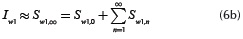
and
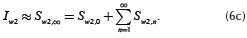
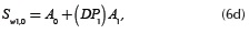
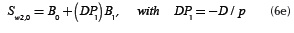
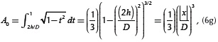
The initial constant terms, Sw1,0 and Sw2,0, are given by
and
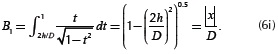
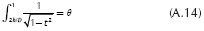
Where
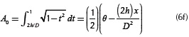
with θ = 0.5π - sin - (2h / D),
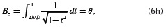
and
Recursive terms Sw1,n and Sw2,n are defined by

and

Where
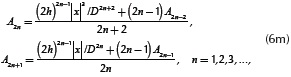
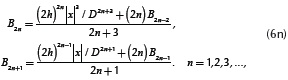
The stopping criterion of Equation (6b) and Equation (6c) is determined when
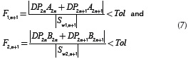
are defined for an absolute error tolerance (Tol). The application of this criterion allows the truncation of the infinite series expansion. The numerical computation of the recursive formula is illustrated in the flowchart shown in Figure 2.
Accuracy and convergence test
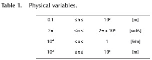
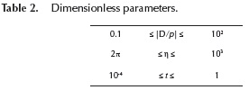
The recursive formula for Sw, described in the previous section as a function of physical and electrical variables (h, x, D, ω, σ and p), is now evaluated for a broad range of parameters to test its accuracy and convergence. To achieve this, the next dimensionless variables are introduced.
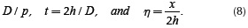
Dimensionless variables relate physical and electrical variables. Table 1 provides the range of values for physical and electrical variables (Uribe et al., 2004). These data are used to establish the ranges of greater practical interest for dimensionless parameters in Equation (8), which are provided in Table 2.
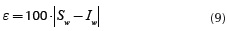
As a first evaluation, the proposed recursive formula for Sw is computed at different values of |D /p| ≤ 60 and 10-3 ≤ η≤ 103. The absolute error tolerance used to stop the computation of Sw is 10-15. The values used for σ= 0.05 S/m and the frequency range has been uniformly sampled from 1 Hz to 1 MHz. The numerical results obtained with the series solution are compared against the numerical integration method 'quadl' (Gander and Gautschi, 2000) of Iw through the absolute percent error (ε):
Here, the results obtained with the numerical integration are used as reference for doing the comparisons. The criterion used to analyze the general series convergence of Sw is determined by the ratio tests.
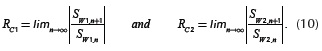
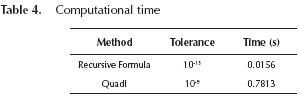
Table 3 provides some simulation results for t = 0.7. It can be observed in the second column of this table that the number of required iterations to reach a good precision is directly proportional to the value of factor |D /p|. The results computed with the numerical integration method 'quadl' are provided in the third column of this table. It is possible to see that its value decreases largely as |D /p| increases. Comparisons between this method and the series solution are provided in the fourth column in the form of maximum absolute percent errors (εmax). These values show that the 1 x max' series expansion method provides accurate computations for up to |D /p| ≤ 30. Oppositely, the series solution becomes very inaccurate for |D /p| > 30. Based on these results the value |D /p| ≤ 30 is proposed as the practical limit to use the series solution for transient response calculations. The series solution of Sw is approximated to zero for |D /p| > 30 due to the fact that Iw is very small.
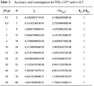
The ratios RC1 and RC2 provided in the fifth column of Table 3 become 1 when the number of iterations tends to N. So, it can be said that the series converges only if |t| < 1. This means that the convergence is guaranteed for the all values of the dimensionless variable t.
A second evaluation to test the accuracy consists of comparing the broad range results between Sw and Iw through a contour map of percent relative error. Figures 3a and 3b provide these results in the form of 3D graphs for the real and imaginary components of Iw . The figures were generated by solving Iw 1000 times. The broad range solution of Sw was evaluated for |D /p| < 30 and approximated to zero for |D /p| > 30. The computational times obtained for DOIng these tasks by an Intel® CoreTM i7-3770 CPU @ 3.40 GHz running MATLAB® V. 7.14 were 0.078 s with the series solution and 5.35 s with the numerical integration.
The contour map depicted in Figure 3c shows the absolute percent errors obtained from the broad range simulation. It can be observed that magnitudes of these errors are always less than 0.01% for |D /p| ≤ 30 and less than 1% by making Sw ≈0. The broad range solution shows that the numerical results provided in Table 3 with t = 0.7 for a particular cable configuration are general. Thus, the criterion of the practical limit to compute Sw can be extended to a broad range of applications.

Case studies
In this section the self and mutual earth return impedances (ZT) are evaluated with three different methods: a) the recursive formula proposed in this paper, b) the numerical integration method "quadl" (Gander and Gautschi, 2000), and c) the approximated formula published by Saad et al. (1996). The validation test consists of comparing the frequency responses obtained with these three methods through the absolute percent error. It should be noted that the numerical integration method is applied for both Pollaczek's integral Equation (3b) and Wedepohl's integral Equation (3d). The latter is considered the reference case for DOIng these comparisons.
Typical case of a power system of buried cables
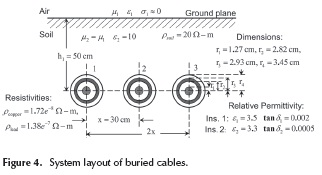
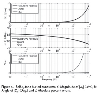
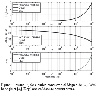
A power system of three cables is used to perform the validation test. Physical variables for this system are depicted in the transversal layout of Figure 4.
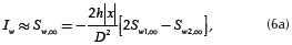
Figures 5 and 6 show, respectively, the plots of self and mutual impedance (ZT) as a function of frequency in terms of its magnitude per unit of length (Ω/m) and the angle in degrees. The setting tolerance used to stop the recursive formula is 10-15 and the tolerance parameter given to the numerical integration is 10e-9. The accuracy of the results was measured with the criterion of absolute percent error. By comparing absolute errors in Figures 6 and 7, one can say that Saad et al (1996) formula gives significant errors, greater than 1%, at high frequency. Oppositely, the recursive formula and the numerical integration give accurate results, smaller than 0.1 % over the entire frequency range. The numerical integration is slightly more accurate than the series algorithm.

Case of AC interference on oil and gas pipelines
There are practical cases in which oil, gas and water pipelines share the same right of way with power transmission systems of aerial lines and buried cables. These cases are a main concern for public utilities because high voltage in power lines and cables can cause AC interference on these pipelines.For instance, during normal operation conditions, power transmission systems induce voltages and currents among their conductors and any other surrounding conducting material in the vicinity. The magnitudes of induced voltages and currents may be greater during abnormal conditions caused by strike lighting and faults.
Part of this energy can be captured by the pipelines and transported along their entire length to the gas stations or water supply valves, which can result in an electrical hazard for people touching the pipelines or metallic structures connected to the pipeline or simply standing nearby. Furthermore, the AC interference can also result in damage to the pipeline and its coating. To predict and mitigate these conditions, it is necessary for electrical engineers to count with tools for the accurate evaluation of earth return impedance.
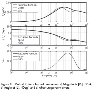
Consider the power transmission of buried cables shown in Figure 7, which is electromagnetically coupled to a petroleum/gas pipeline. The ground resistivity is 20 Ω2-m. For the calculation of mutual electromagnetic couplings among conductors 3 and 4, consider a horizontal distance of 30 meters and a depth of 0.50 m for both conductors.
Figure 8 shows the plot of mutual impedance (ZT) plots as a function of frequency in terms of its magnitude per unit of length (Ω/m) and the angle in degrees. For this case, the frequency range has been logarithmically spaced from 10 Hz to 1 MHz by using 100 points per decade. Frequency responses for ZT have been calculated with the recursive formula, the numerical integration 'quadl' and the Saad et al. formula (1996). By comparing the three methods used one can say that the approximated formula gives significant errors in high frequency. In contrast, the recursive formula and the numerical integration 'quadl' give the same accuracy over the entire frequency range. However, the main advantage of the recursive formula over the numerical integration 'quadl' is its low computational demand. Table 4 provides the computational time required for both methods with an Intel® CoreTM i7-3770 CPU @ 3.40 GHz running MATLAB® V. 7.14. It can be observed that the recursive formula is faster than the numerical integration method.
Transient study
The inverse Numerical Laplace Transform (NLT) technique is used as a reference tool to calculate the open circuit transient response in the time domain (Uribe et al, 2002). The recursive formula and the numerical integration have been incorporated into the CABLE toolbox of the NLT technique for evaluating the frequency-dependent parameter ZT. The open circuit transient response is also calculated with the real-time platform RSCAD/RTDS®. The CABLE program of this platform has been adjusted to evaluate ZT with the numerical integration and the transient calculation with the frequency dependent model. The aim of this section is to compare the transient responses obtained with NLT and the commercial real-time platform RSCAD/RTDS®.
Open circuit test
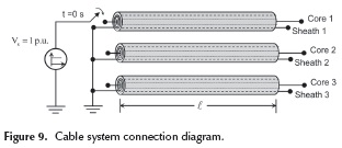
Consider the three-phase buried cable system whose data is provided in Figure 4. A unit step voltage of 1 p.u. is applied at t = 0 s to the core of cable 1 as shown in Figure 9. At the sending end, the cores of cables 2 and 3 are left in open circuit while sheaths are short-circuited. At the receiving end, all conductors are left open. The time step to perform this simulation test is 10 us, as this is the minimum allowed by RSCAD/RTDS® with the full frequency-dependent cable model. The NLT technique uses an observation time of 3 ms with 1000 samples to match the simulation time-step.
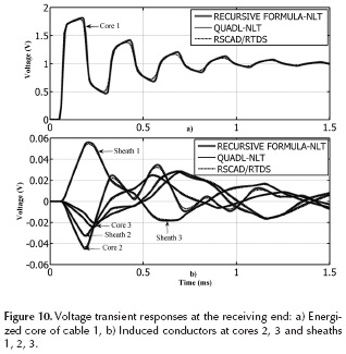
The voltage transient response at the receiving end for the energized core of cable 1 is depicted in Figure 10a, while induced voltages for cores 2 and 3, and sheaths 1, 2 and 3 are depicted in Figure 10b. The open circuit transient responses obtained through the inverse NLT technique with the recursive formula and the numerical integration match exactly the same behavior. Absolute errors between these waveforms are less than 10-4. However, voltage waveforms captured from the real-time simulation in RTDS present some small discrepancies with the NLT technique. These small differences are probably due to larger time-steps and do not represent the full frequency dependence of parameters. For instance, a time-step of 10 us corresponds to an effective bandwidth of 15 kHz. To have a good resolution of the transient response in the time domain it is necessary to perform the simulation with time-steps smaller than 10 µs.
Conclusions
An accurate, efficient and reliable methodology to evaluate the earth return impedance on buried cables for a broad range of frequencies and cable configurations has been presented in this paper. This methodology differs considerably from traditional methods, numerical integration and approximate formulas, because ZT is computed exclusively by means of infinite series through a recursive formula. The proposed method uses the analytical decomposition derived by Wedepohl and Wilcox (1973) to transform Pollaczek's integral into a set of improper integrals plus a definite integral. The improper integrals are computed fast and easily in modern mathematical tools when they are approximated to an infinite series of Bessel functions. The main contribution of this paper has been the development of a recursive formula based on infinite series for computing the definite integral or Wedepohl-Wilcox's integral. It has been demonstrated that the recursive formula provides enough accuracy for a broad range of frequencies and cable configurations. By comparing this method with the algorithms reported by Wedepohl and Wilcox (1973) and by Uribe and Ramirez (2012), it can be said that the range of application has been extended. This is mainly because the recursive formula can provide accurate results for up to |D / p| ≤ 30. Furthermore, its execution in a conventional PC is always faster than the numerical integration method. This reliable method can be incorporated in CABLE routines of electromagnetic transients programs such as the NLT technique and the real-time platform RSCAD/RTDS®.
Appendix A
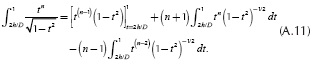
The method of integration by parts is used to evaluate integrals An in Equation (5a) and Bn in Equation (5b). Its general formula is given by
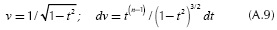
The following variables are defined:
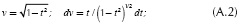
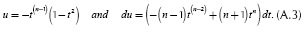
By substituting these variables in Equation (A.1),
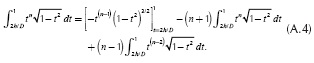
and by regrouping identical terms.
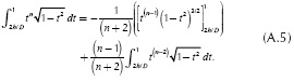
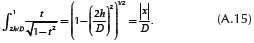
Then, by evaluating upper and lower integration limits
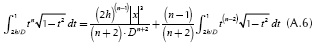
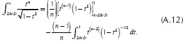
where |x|/D is defined by  according to the geometric relations shown in Figure 1. The exponent n comes from the series expansion defined in (4d). Thus, this integral has to be evaluated N+1 times from n = 0 to n = N. The evaluation of Equation (A.6) can be handled recursively because it depends on its past values. In order to find the recursive series solution for Equation (A.6), the first two terms are computed. For n = 0,
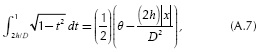
with θ = 0.5Π-sin-(2h/D) and for n = 1
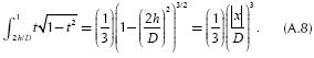
The solution of Equations (A.7) and (A.8) corresponds to the initial constant terms of the series expansion. Now, the same procedure is done for Equation (5.b). The following variables are defined

By replacing Equations (A.9) and (A.10) in Equation (A.1),
By regrouping identical terms, Equation (A.11) becomes
By evaluating upper and lower integration limits,
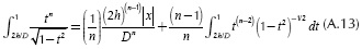
where |x|/D is defined by . Finally, by evaluating Equation (A.13) for n = 0 and n = 1
Appendix B
This Appendix shows some critical cases to demonstrate the accuracy of the recursive formula proposed in this paper.
Poor conducting soil
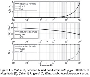
The mutual impedance ZT between cables 1 and 2 of the system layout depicted in Figure 5 is calculated with a soil resistivity of 1000 Ω-m. The simulation results are depicted in Figure 11. The absolute percent errors obtained with a high soil resistivity have the same magnitudes than those obtained with a good conducting soil (20 Ω-m).
Worse case for the numerical integration
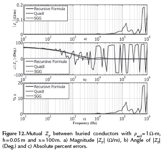
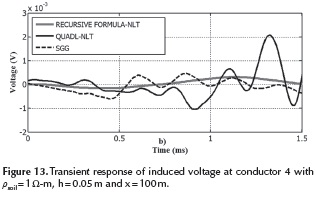
The mutual impedance ZT between cable 1 and conductor 4 of the system layout depicted in Figure 7 is calculated with a soil resistivity of 1 Ω-m. The depth of the cable and the conductor is 0.05m and the horizontal distance between cable and conductor is 100 m. The simulation results are depicted in Figures 12 and 13. Opposite to Figure 8, it can be seen that the numerical integration fails considerably along the entire frequency range. Also, the approximated formula gives significant errors in the zone of low frequency. The computation of ZT with critical cases of buried cables may cause significant differences in the time domain transient response. For that reason, it is essential to count with a reliable methodology to calculate ZT for a broad range of frequencies and cable configurations.
Acknowledgment
The authors gratefully acknowledge the support of the National Council of Science and Technology of Mexico (CONACYT) and the Center for Research in Mathematics A.C. (CIMAT).
References
Ametani, A. (1980). A general formulation of impedance and admittance of cables. IEEE Transactions on Power Apparatus Systems, PAS-99(3), 902-910. DOI: 10.1109/TPAS.1980.319718. [ Links ]
Carson, J. (1926). Wave Propagation in Overhead Wires with Ground Return. Bell System Technical Journal, 5(4), 539554. DOI: 10.1002/j.1538-7305.1926.tb00122.x. [ Links ]
Deri, A., Tevan, G., Semlyen, A., and Castanheira, A. (1981). The complex ground return plane: A simplified model for homogeneous and multi-layer earth return. IEEE Transactions on Power Apparatus and Systems, PAS-100(8), 3686-3693. DOI: 10.1109/TPAS.1981.317011. [ Links ]
Dommel, H. W. (1986). Electromagnetic Transients Program Reference Manual (EMTP Theory Book), Prepared for Bonneville Power Administration, P.O. Box 3621, Portland, Ore., 97208, USA. [ Links ]
Dubanton, C. (1969). Calcul approaché des parametrés primaires et secondaires d'une ligne de transport-Valeurs homopolaires. E. D. F., Bulletin de la Direction des Études et Recherchches No. 1, sere B. [ Links ]
Gander, W., and Gautschi, W. (2000). Adaptive Quadrature-Revisited. BIT, 40(1), 84-101. DOI : 10.1023/A:1022318402393. [ Links ]
Gary, C. (1976). Approche complète de la propagation multifilaire en haute fréquence par utilisation des matrices complèxes. E.D.F Bulletin de la Direction des Études et Recherches, Série B (3/4), 5-20. [ Links ]
Legrand, X., Xemard, A., Fleur, G., Auriol, P., Nucci, C.A. (2008, July). A Quasi-Monte Carlo Integration Method Applied to the Computation of the Pollaczek Integral. Power Delivery, IEEE Transactions on, 23(1), 1527-1534. [ Links ]
Nguyen, T.T. (1998, November). Earth-return path impedances of underground cables. I. Numerical integration of infinite integrals. Generation, Transmission and Distribution, IEE Proceedings, 145(6), 621-626. DOI: 10.1049/ip-gtd:19982353. [ Links ]
Papagiannis, G.K., Tsiamitros, D.A., Labridis, D.P., Dokopoulos, P.S. (2005, May). Direct numerical evaluation of earth return path impedances of underground cables. Generation, Transmission and Distribution, IEE Proceedings, 152(3), 321-327. DOI: 10.1049/ip-gtd:20045011. [ Links ]
Pollaczek, F. (1926). Über das Feld einer unendlich langen Wechsel stromdurchflossenen Einfachleitung. Electrische Nachrichten Technik, 3(9), 339-360. [ Links ]
Saad, O., Gaba, G., Giroux, M. (1996, July). A closed-form approximation for ground return impedance of underground cables. IEEE Transactions on Power Delivery, 11(3), 1536-1545. DOI: 10.1 109/61.517514 [ Links ]
Semlyen, A. (1985, February). Discussion to overhead Line parameters from handbook formulas and computer programs by H. Dommel. IEEE Trans. on Power Apparatus and Systems, PAS-104(1), 371. [ Links ]
Theodoulidis, T. (2012, August). Exact Solution of Pollaczek's Integral for Evaluation of Earth-Return Impedance for Underground Conductors. Electromagnetic Compatibility, IEEE Transactions on, 54 (4), 806-814. [ Links ]
Uribe, F. A., Naredo, J. L., Moreno, P., and Guardado, L. (2002). Electromagnetic Transients in Underground Transmission Systems Through The Numerical Laplace Transform. Elsevier Science Ltd, Electrical Power and Energy Systems, 24(1), 215-221. DOI: 10.1016/S0142-0615(01)00031-X. [ Links ]
Uribe, F. A., Naredo, J. L., Moreno, P., and Guardado, L. (2004, January). Algorithmic evaluation of underground cable earth impedances. IEEE Transactions on Power Delivery, 19(1), 316-322. DOI: 10.1109/TPWRD.2003.820181. [ Links ]
Uribe, F.A., Ramirez, A. (2012, October). Alternative Series-Based Solution to Approximate Pollaczek's Integral. Power Delivery, IEEE Transactions on, 27(4), 2425-2427. [ Links ]
Wedepohl, L. M., and Wilcox, D.J. (1973). Transient analysis of underground power transmission systems. Proceedings of the IEE, 120(2), 253-260. [ Links ]
Zou, J., JunJie, Li, Lee, J. B., Chang, S. H. (2011, February). Fast and Highly Accurate Algorithm for Calculating the Earth-Return Impedance of Underground Conductors. Electromagnetic Compatibility, IEEE Transactions on, 53(1), 237-240. [ Links ]
