DOI: http://dx.doi.org/10.15446/ing.investig.v35n1Sup.53673

Fault location in power distribution systems considering a dynamic load model

Localización de fallas en sistemas de distribución de energía eléctrica considerando un modelo dinámico de carga

D. Patiño-Ipus¹, H. Cifuentes-Chaves², and J. Mora-Flórez³

¹ Daniel Fernando Patiño Ipus: B.Sc. in Electrical Engineering from the Universidad Tecnológica de Pereira, Colombia.
E-mail: danferpatino@utp.edu.co
² Harold Andrés Cifuentes Chaves: B.Sc. in Electrical Engineering from the Universidad Tecnológica de Pereira and M.Sc candidate in Electrical Engineering from the Universidad Tecnológica de Pereira, Colombia.
E-mail: hacifuentes@utp.edu.co
³ Juan José Mora Flórez: B.Sc. and M.Sc. in Electrical Engineering from the Universidad Industrial de Santander, Colombia. Ph.D. in Electrical Engineering from the Universitat de Girona, España. Affiliation: Associated professor at Universidad Tecnológica de Pereira, Colombia.
E-mail: jjmora@utp.edu.co

How to cite: Patiño-Ipus, D., Cifuentes-Chaves, H., & Mora-Flórez, J. (2015). Fault location in power distribution systems considering a dynamic load model. Ingeniería e Investigación, 35(Supl), 34-41. DOI: http://dx.doi.org/10.15446/ing.investig.v35n1Sup.53673

ABSTRACT

In the electrical power systems, load is one of the most difficult elements to be represented by an adequate mathematical model due to its complex composition and dynamic and non-deterministic behavior. Nowadays, static and dynamic load models have been developed for several studies such as voltage and transient stability, among others. However, on the issue of power quality, dynamic load models have not been taken into account in fault location. This paper presents a fault location technique based on sequence components, which considers static load models of constant impedance, constant current and constant power. Additionally, an exponential recovery dynamic load model, which is included in both the fault locator and the test system, is considered. This last model is included in order to consider the dynamic nature of the load and the performance of the fault locators under this situation. To demonstrate the adequate performance of the fault locator, tests on the IEEE 34 nodes test feeder are presented. According to the results, when the dynamic load model is considered in both the locator and the power system, performance is in an acceptable range.

Keywords: Fault location, electric power distribution systems, power quality, dynamic load model.

RESUMEN

En los sistemas eléctricos de potencia, la carga es uno de los elementos matemáticamente más difíciles de representar debido a su compleja composición y su comportamiento dinámico y no determinístico. Actualmente, se han desarrollado modelos estáticos y dinámicos de carga para diversos estudios, tales como estabilidad de tensión y estabilidad transitoria, entre otros. Sin embargo, en el campo de la calidad de la energía no se han tenido en cuenta los modelos dinámicos en la localización de fallas. Este artículo presenta una técnica de localización de fallas basada en componentes de secuencia, que considera modelos estáticos de impedancia constante, corriente constante y potencia constante. Además, se considera un modelo dinámico de recuperación exponencial, tanto en el localizador como en el sistema de pruebas. Este modelo se incluye para considerar la naturaleza dinámica de la carga y el desempeño de los localizadores ante esta situación. Para demostrar el desempeño adecuado del localizador de fallas, se realizaron pruebas en el sistema IEEE de 34 nodos. De acuerdo con los resultados, cuando se considera el modelo dinámico tanto en el localizador como en el sistema, el desempeño está en un rango aceptable.

Palabras clave: Localización de fallas, sistemas de distribución de energía, calidad de la energía, modelos dinámicos de carga.

Received: September 15th 2015 Accepted: October 10th 2015

Introduction

Power quality includes the quality of the energy supplied and the customer service. Quality of supply is related to the waveform and continuity. An efficient and timely fault location enables power utilities to improve service continuity indices (Mora, 2006).

On the other hand, load can be widely defined as one network device that absorbs, generates or controls active and reactive energy, which is affected by power system variations in voltage and frequency (Rifaat, 2004). In accordance with (Romero, 2002), in order to select an appropriate load model the load composition and disturbances behaviour must be previously known.

Moreover, impedance based fault location techniques are highly dependent on the power system representation (Mora, 2006). Thus, by using models which accurately represent the behaviour of the power system elements, these methods could improve its performance.

Nowadays, transmission lines, electrical generators and power compensators, among other devices, have acceptable models (Rodriguez, et al., 2013). However, an appropriate load model is difficult to obtain due to the large number and diversity of the elements at the power distribution system (Chiang, et al., 1996). Besides, load variations over time and inaccurate information about load composition make this work complex (Stojanovi'c, et al., 2007). Therefore, an appropriate load model that represents variations over time and is simultaneously suitable to be used in fault location methods is needed. In order to obtain a realistic representation of the power system and more operating scenarios in the fault location, the inclusion of the load model is analysed in this paper.

Taking into account the dynamic behaviour of the electrical loads, this paper proposes a fault location technique which considers static and dynamic load models in both the locator and the test power distribution system. This new approach allows to obtain a better power distribution system, modelled for more realistic tests. Finally and according to the documentation analysis, dynamic load models were not included in previous studies of fault location, as these presented in (Roman, 2014), (Herrera, 2013), (Bedoya, 2013), (Bedoya Cadena, et al., 2013), (Panesso, et al, 2015), (Orozco, et al., 2013), (Brahma, 2011), (Mora, 2006), (Das, 1998) and (Hagh, et al., 2012).

The proposed technique was tested with all shunt fault types (single phase to ground, phase to phase, and three phase), considering different distances from the main power substation, several fault resistances (Rf), and variations on the load model (Constant impedance, constant current, constant power, and dynamic models).

In the second section of this paper, the theoretical aspects for fault location using different dynamic load models are presented. In the following section, the exponential recovery load model was developed to consider it into the fault locator. The fourth section proposes the general methodology developed. Tests on the IEEE34 power system are then presented in section five. Finally, the most important conclusions are presented in the last section.

Theoretical basic aspects

This section is devoted to present the basic concepts used in this paper; detailed information can be obtained consulting the provided references.

Fault location method

The proposed fault location technique is based on the method developed in (Bedoya, et al., 2013). The technique is defined in Figure 1, where a line section between the nodes (x) and (y) of a faulted power distribution feeder is shown.

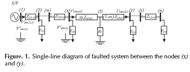
Where,

: Phase voltage in fault steady state, at node (x).

: Phase current in fault steady state, flowing from node (x) to node (f).

: Phase line section impedance from node (x) to node (y).

: Load admittance matrix at node (x).

: Per-unit fault distance based on the line section length.

: Fault resistance.

A sequence equivalent power system was developed for each type of fault: single phase to ground, phase to phase, and three phase faults. Afterthis, a second order polynomial equation for each type of fault is obtained.

The general equation for the fault location is presented in Equation (1), where the constants Kα, Kb, Kc and Kd are a function of the power system parameters in Figure 1.

Expression (1) is separated into real and imaginary parts. Then, two equations with two unknowns (R_f and m) are obtained. Finally, solving this equation the m value is estimated.

Load models

Static load models represent the active and reactive power as an algebraic function of the nodal voltage and/or the system frequency at the same time instant. Equations (2) show the general representation.

A general load model is the ZIP model, which represents the active and reactive power as a polynomial equation. Equations (3) and (4) contain the combined effect of load models of constant impedance, constant current and constant power.

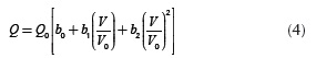
Where P_o, Q_o is the rated active and reactive power, is the per unit load voltage, and finally, α₀ α₁, α₂, b₁, b₂ are the constant impedance, constant current and constant power coefficients of the active and reactive power, respectively. These coefficients meet the relations shown in Equations (5) and (6).

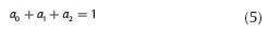
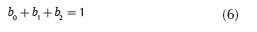
Moreover, different load models can be obtained from Equations (3) and (4), assuming coefficients values as:

α₀=b₀=1 Constant power.

α₁=b₁=1 Constant current.

α₂=b₂=1 Constant impedance.

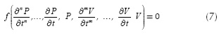
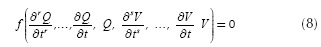
On the other hand, dynamic load models represent the active and reactive power through differential equations or difference equations, as functions of the absolute voltage and the system frequency. Equations (7) and (8) show the general representation.

The exponential recovery load model, which is a dynamic model used in this paper, was experimentally developed from load behaviour analysis in substations under voltage disturbances (Karlsson & Hill, 1994). Equations (9) and (10) show the mathematic representation of the model.

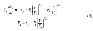
Where,

: State variables for active and reactive power, p ^{q 1} respectively.

: Exponential recovery time for active and reactive power, respectively.

: Exponents associated with steady state load response.

: Exponents associated with transient load response.

: Rated active and reactive power, respectively.

: Active and reactive power demand of the load.

: Load voltage.

: Load voltage in prefault steady state

Numerical methods to solve the dynamic load model

Some of the most popular methods to solve the differential equations of the load model are briefly discussed in this section.

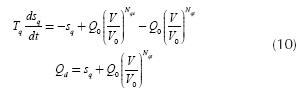
1. Euler method

This method uses the derivative of a function y(x), evaluated at a point x₀ as the slope of the tangent line at this point. Therefore, if a short distance is travelled along this tangent line, then it can be getting an approximation to the real solution (Zill, 1997). The equations are presented in Equation (11).

Where h is the step size, x₀ are the initial conditions, y₀ are the previous states and x_n-1' y_n-1 are the previous states and x_n-1' y_n-1 are the current states.

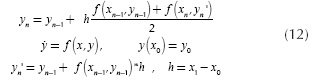
2. Improved Euler method

This method calculates an average gradient between the current state and the next one. This method provides a better approximation than the previous one, according to (Zill, 1997). Equations for this method are presented in Equation (12).

3. Runge-Kutta method

This method is widely used due to its high precision, which was developed through the Taylor series (Zill, 1997). General equations for the fourth order method are presented in Equation (13).

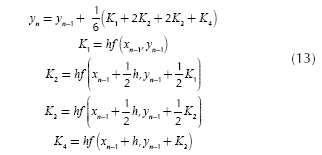
Where K₁, K₂, K₃ and K₄ are the constants of the method.

Load representation using the exponential recovery load model

The purpose of this section is to present the strategy used to include the dynamic behaviour of the load inside the code of the fault locators, which was done by updating voltage and current for each line section under study. The proposed method consists in modifying the equations, which describe the active and reactive power behaviour. Thus, these new modified equations describe the active and reactive admittance behaviour, which depends on the voltage variations.

The here presented development of the load representation is only for the active power; however, it is similar for the reactive power. The new equations are the results of dividing Equation (9) by the square load voltage, as follows:

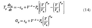
With

After this, Equation (14) is multiplied and divided by the square load voltage in prefault steady state. When organizing the equation, an expression for the admittance as a function of the exponential recovery load model is obtained, as presented in Equation (15). Similarly, the same process is done for the reactive power.

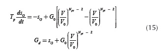
with

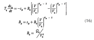
Where,

S_G, S_B: State variables associated with active and reactive admittance.

G₀, B₀: Rated admittance related with the active and reactive

G_d, B_d: Load admittance related with the active and reactive power, respectively.

Similarly, it is possible to obtain an expression of the load admittance for the ZIP model.

Proposed methodology

The flowchart of the proposed methodology used to obtain the specific load model and to include it at the fault location method is depicted in Figure 2. Following, the stages are described:

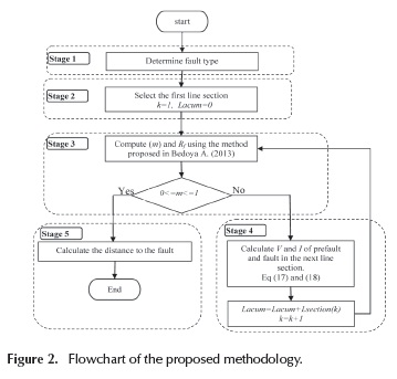
Stage 1. Determine the fault type

The fault type is determined using the algorithm proposed by (Das, 1998).

Stage 2. Select the first line section

The proposed methodology developed in (Bedoya, et al., 2013), proposes an iterative process, which begins with the selection of the first line section as the faulted section.

Stage 3. Application of the fault location method

In this stage, the fault location technique is applied to obtain the distance to the fault (m). The m value corresponds to a per unit distance in the analysed line section. If the m value is between 0 and 1, then the actual section could be the faulted section. Otherwise, the next line section is analysed. Finally, the fault location method obtains the distance from the substation to the fault.

Stage 4. Updating of voltage and current of the next line section

Normally, the measurements are only available in the power distribution system and are associated with the main power substation. Therefore, an iterative sweep section by section is performed for updating voltage and currents in fault conditions on the others line sections. This process is shown in Figure 3.

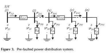
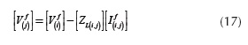
To compute the voltage and current at node (j), shown in Figure 3, from voltage and current measured in the main power substation, Equations (17) and (18) are used, respectively.

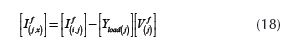
Where,

: Phase voltages in fault condition at the node (i)

: Phase voltages in fault condition calculated at the node (j)

: Phase currents in fault condition between (i) and (j)

: Phase currents in fault condition between (j) and (x)

: Phase line section impedance from node (i) to node (j).

: Phase load admittance at node (j).

In Equation (18), the load effect in the load admittance dependence can be observed. This effect comprises either individual loads or equivalent circuits. The integration of the load models in the fault location technique is performed in this section through the following 4 phases described below:

PHASE 1: Load model identification

In this phase, the model representing the load connected to the node under consideration is defined. There are two possibilities:

• Static model (ZIP)
• Dynamic model (Exponential recovery load model) PHASE 2: Load model solution

At this phase, the active and reactive power load is obtained. For this phase there are two cases:

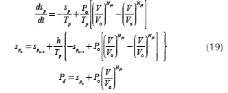
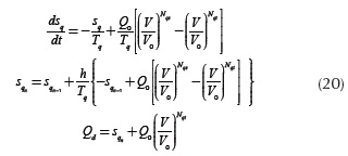
In the case of a static model, the P and Q values are directly obtained from the model Equations (3) and (4). Otherwise, in case of a dynamic model, a numerical method is applied to solve the differential equations and to obtain P and Q. In this paper, an Euler method is applied to the exponential recovery load model due to its easily programming, and to obtain Equation (19), which is the solution of Equation (9). Similarly, for the case of reactive power, Equation (20) is obtained.

PHASE 3: Getting load admittance as a function of P and Q

At this phase, the load admittance connected in the node under consideration is obtained as a function of P and Q. These P and Q values contain the static or dynamic load behaviour. The expression for load admittance is obtained by applying the technique shown in section 3 to Equations (19) and (20).

PHASE 4: Updating of voltage and current considering the load models

At this phase, Equations (17) and (18) are used with the load admittance computed in the previous phase in order to update the voltages and currents downstream the analysed section.

Stage 5. Calculate distance to the fault

The total distance to the fault is computed with the addition of the previous line section lengths and the percentage of the line section under fault related to m. This distance is computed with Equation (21).

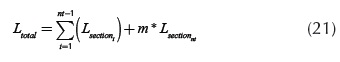
Where,

L_est: Total distance from substation to the faulted node.

nt: Number of studied line section.

: Length of the last analysed line section.

Tests and results

Test system

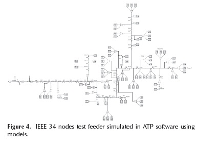
The system selected is the 24.9 kV IEEE 34 nodes test feeder, shown in Figure 4 This is simulated using ATP power simulator. This power distribution system has single and three phase laterals, unbalanced loads and different lengths and configurations of the line sections. This power system was modified to include the here analysed load models.

Test scenarios

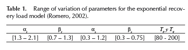
The considered load models are constant impedance (Zcte), constant current (Icte), constant power (Scte), hybrid model, and the exponential recovery load model. For the exponential recovery load model, the parameters used are those presented in (Romero, 2002). The variation range of these parameters is the shown in Table 1.

To validate the methodology, four different test scenarios are proposed.

a) First scenario

Test system at the rated operating conditions, with ZIP static load model. The fault locator does not take into account the ZIP static load models, but, instead, a constant impedance model is used.

b) Second scenario

Test system is considered at the rated operating conditions, with ZIP static load models. The fault locator takes into account the ZIP static load models.

c) Third scenario

Test system is considered at the rated operating conditions, with the exponential recovery load model. The fault locator does not contain the dynamic model; instead, a constant impedance (Zct) model is used.

d) Fourth scenario

Test system at the rated operating conditions together with the exponential recovery load model is considered at this scenario. The fault locator takes into account the dynamic model.

In all of the proposed scenarios, single-phase, two-phase and three-phase faults with different fault resistances between 0-40Ω are considered (Dagenhart, 2000). Constrained by the paper length, only the results for single-phase faults will be displayed in the four proposed scenarios.

Results analysis

The performance of the proposed fault location technique is defined by an absolute error indicator, as presented in Equation (22).

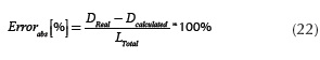
Where D_Real is the real distance from the power substation to the faulted node, D_calculated corresponds to the estimated distance by the fault locator and L_Total is the total length of the equivalent radial.

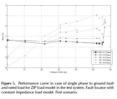
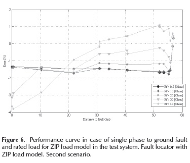
According to Figure 5, the power system with the ZIP load model presents the highest error in fault location (-4 %), considering Rf equal to 40Ω. The performance curves in this case show an error between -4.0 °% and 2 °%. In Figure 6, the errors range from -4.0 °% to 2 °%, considering ZIP load models in both the test system and the fault locator. This response is similar to the previous one, which was expected.

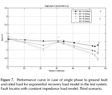
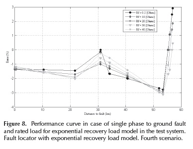
Additionally, in Figure 7 the higher error range is from -3.0 % to 0.5 %, considering the exponential recovery load model in the test system, but not in the fault locator. In this case, the performance is better than the first scenario, due to better load representation obtained with the dynamic load model. Finally, in Figure 8 the errors rangefrom -4.0 % to 3 %, considering the exponential recovery load model in both the test system and the fault locator. This response was not expected, but it fits into an acceptable range.

The two-phase faults for the four scenarios present a higher error range, from -1.5 % to 3%. Furthermore, the three-phase faults present a higher error range from -2.0 °% to 3 °%. These errors are in an acceptable range for fault location.

In Table 2, a summary of the results for all test scenarios is presented. It can be observed that a lower total error is presented when the test power system has a better representation, which includes the dynamic phenomena.

Conclusions

A fault locator method that considers an exponential recovery dynamic load model was presented. The performance obtained for the proposed fault location technique considering dynamic load models is high, taking into account that the errors obtained are lower than 4 %%.

Finally, the consideration of the real load models helps to improve the performance of the fault locator, providing a useful tool to improve the supply continuity at power distribution utilities.

Acknowledgments

This research was supported by the Universidad Tecnológica de Pereira (Colombia) and COLCIENCIAS, under the project "Desarrollo de localizadores robustos de fallas paralelas de baja impedancia para sistemas de distribución de energía eléctrica LOFADIS 2012", contract number 0977-2012; and the Master program in Electrical Engineering, Universidad Tecnológica de Pereira (Colombia).

References

Bedoya. A., Mora J., Perez S., (June 2013). Extended application of a sequence impedance based fault location technique applied to power distribution systems. Dyna rev. fac. nac. minas. vol.80 no.179 Medellín.         [ Links ]

Bedoya-Cadena, A., Mora-Flórez, J. and Pérez-Londoño, S. (2012). Estrategia de reducción para la aplicación generalizada de localizadores de fallas en sistemas de distribución. EIA Journal, Vol 17.         [ Links ]

Bedoya, A. (2013). Estrategia generalizada para la aplicación de métodos de localización de fallas basados en la estimación de la impedancia o MBM. Master thesis, Universidad Tecnológica de Pereira, Pereira, Colombia.         [ Links ]

Bedoya Cadena, Andrés and Mora Flórez, Juan and Pérez Londoño, Sandra (2013) Aplicación extendida de una técnica de impedancia de secuencia a la localización de fallas en sistemas de distribución. Dyna; Vol. 80, núm. 179 (2013); 157-164.         [ Links ]

Brahma, S.M. (July 2011). Fault Location in Power Distribution System With Penetration of Distributed Generation. Power Delivery, IEEE Transactions on. vol. 26, no 3, pp. 1545 - 1553.         [ Links ]

Chiang, Hsiao-Dong., Wang, Jin-Cheng., Huang, Chiang-Tsung., Chen, Yung-Tien., and Huang, Chang-Horng. (1997). Development of a Dynamic ZIP-Motor Load Model From On-Line Field Measurements. Electrical Power & Energy Systems, Vol. 19, No. 7, pp. 459-468, Received 18 September 1996; accepted 19 December. DOI: 10.1016/S0142-0615(97)00016-1.         [ Links ]

Das, R. (1998). Determining the locations of Faults in distribution systems. Doctoral Thesis University of Saskatchewan, Saskatoon, Canada, sprina.         [ Links ]

Dagenhart, J. (2000). "The 40ohms ground-fault phenomenon", IEEE Transactions on Industry Applications, 36(1), p 30-32. DOI: 10.1109/28.821792        [ Links ]

Hagh, M.T.; Hosseini, M.M.; Asgarifar, S. (May 2012). A novel phase to phase fault location algorithm for distribution network with distributed generation Integration of Renewables into the Distribution Grid, CIRED 2012 Workshop, pp. 1-4.         [ Links ]

Herrera R., O. (2013). Análisis de los Efectos de la Variación de los Parámetros del Modelo de Línea, de Carga y de Fuente, en la Localización de Fallas en Sistemas de Distribución. Master thesis, Universidad Tecnológica de Pereira, Pereira, Colombia.         [ Links ]

IEEE Distribution System Analysis Subcommittee. Radial Test Feeders. (2000) http://www.Ewh.ieee.org/soc/pes/sacom/testfeeders.html. DOI: 10.1109/59.317546.         [ Links ]

Karlsson D. and Hill D. J. (Feb. 1994). Modelling and identification of nonlinear dynamic loads in power systems. IEEE Trans. Power Systems, vol.9, no.1, pp.157-166.         [ Links ]

Mora, J. J. (2006). Localización de Faltas en Sistemas de Distribución de Energía Eléctrica usando Métodos Basados en el Modelo y Métodos Basados en el Conocimiento. Doctoral thesis. Universitat de Girona. Spain.         [ Links ]

Orozco Henao, Cesar augusto and Mora Flórez, Juan José and Pérez Londoño, Sandra (2013) Estrategia iterativa de ajuste de carga aplicada a localización de fallas en sistemas de distribución de energía. Dyna; Vol. 80, núm. 177 (2013); 59-68.         [ Links ]

Panesso-Hernández, Andres Felipe; Mora-Flórez, Juan; Pérez-Londoño, Sandra (2015). Complete power distribution system representation and state determination for fault location. DYNA, [S.l.], v. 82, n. 192, p. 141-149, aug. 2015. ISSN 2346-2183. DOI: dyna.v82n192.48589.         [ Links ]

Rifaat, R.M. (2004).On composite load modelling for voltage stability and under voltage load shedding, In Proc. IEEE Power Engineering Society General Meeting, pp.1603-1610.         [ Links ]

Rodríguez L., Pérez S., Mora J. (Oct, 2013). Estimación de Parámetros de un Modelo de Carga de Recuperación Exponencial Empleando Técnicas Metaheurísticas. Scientia et Technica XVIII, vol.18, no.3, pp.453-462. Universidad Tecnológica de Pereira.         [ Links ]

Román L., M. (2014). Método de Localización de Fallas Considerando el Efecto de la Carga, para Sistemas de Distribución de Energía con Generación Distribuida. Bachelor thesis. Universidad Tecnológica de Pereira, Pereira, Colombia.         [ Links ]

Romero I., N., (2002). Dynamic Load Models for Power Systems, Estimation of Tyme-Varying Parameters During Normal Operation. Doctoral thesis. Departament of Industrial Electrical Engineering and Automation, Lund University, Sweden.         [ Links ]

Stojanovi'c, D. P., Korunovi'c, L. M., and Milanovi'c, J. V. (2007). Dynamic Load Modelling Based on Measurements in Medium Voltage Distribution Network. Electric Power Systems Research 78 (2008) 228.238, Received 11 September 2006, accepted 8 February 2007, Available online 28 March 2007.         [ Links ]

Zill D., G., (1997). Ecuaciones diferenciales con aplicaciones de modelado. Book. Sixth edition.         [ Links ]