DOI: http://dx.doi.org/10.15446/ing.investig.v35n1Sup.53577

Validation of a non-uniform meshing algorithm for the 3D-FDTD method by means of a two-wire crosstalk experimental set-up

Validación de un algoritmo de enmallado para el método 3D-FDTD por medio de un montaje experimental de diafonía de dos conductores

E. Jiménez-Mejía¹, and J. Herrera-Murcia²

¹ Raúl Esteban Jiménez Mejía: Electrical Engineer, Magister in Electrical Engineering, Universidad Nacional de Colombia. Affiliation: Graduate Student, Facultad de Ciencias, Physics Department, Universidad Nacional de Colombia, Medellín, Colombia.
E-mail: rejimene@unal.edu.co
² Javier Gustavo Herrera Murcia: Electrical Engineer, Magister in Electrical Engineering and PhD in Engineering, Universidad Nacional de Colombia, Colombia. Affiliation: Associate Professor, Mines Faculty, Electrical Energy and Automation Department, Universidad Nacional de Colombia, Medellín, Colombia.
E-mail: jherreram@unal.edu.co

How to cite: Jiménez-Mejía, E., & Herrera-Murcia, J. (2015). Validation of a non-uniform meshing algorithm for the 3D-FDTD method by means of a two-wire crosstalk experimental set-up. Ingeniería e Investigación, 35(Supl), 98-103. DOI: http://dx.doi.org/10.15446/ing.investig.v35n1Sup.53577

ABSTRACT

This paper presents an algorithm used to automatically mesh a 3D computational domain in order to solve electromagnetic interaction scenarios by means of the Finite-Difference Time-Domain -FDTD- Method. The proposed algorithm has been formulated in a general mathematical form, where convenient spacing functions can be defined for the problem space discretization, allowing the inclusion of small sized objects in the FDTD method and the calculation of detailed variations of the electromagnetic field at specified regions of the computation domain. The results obtained by using the FDTD method with the proposed algorithm have been contrasted not only with a typical uniform mesh algorithm, but also with experimental measurements for a two-wire crosstalk set-up, leading to excellent agreement between theoretical and experimental waveforms. A discussion about the advantages of the non-uniform mesh over the uniform one is also presented.

Keywords: Finite-difference time-domain (FDTD) method, non-uniform orthogonal mesh, thin-wire models, crosstalk effect.

RESUMEN

Este trabajo presenta un algoritmo usado para enmallar automáticamente un dominio computacional 3D con el fin de solucionar escenarios de interacción electromagnética por medio del Método de Diferencias Finitas en el Dominio del Tiempo - FDTD. El algoritmo propuesto se ha planteado en una forma matemática general, donde es posible definir funciones convenientes de espaciado aplicadas a la discretización del espacio de simulación. Esto permite la inclusión de objetos pequeños en el método FDTD y el cálculo de variaciones detalladas del campo electromagnético en regiones especificadas del dominio de cálculo. Los resultados obtenidos mediante el método FDTD con el algoritmo propuesto se han contrastado no sólo con un algoritmo típico de enmallado uniforme, sino también con medidas experimentales para un montaje de diafonía de dos hilos conductores logrando una excelente concordancia entre las formas de onda teóricas y experimentales. Además, se presenta una discusión sobre las ventajas del enmallado no uniforme sobre el uniforme.

Palabras clave: Método de diferencias finitas en el dominio del tiempo - FDTD, enmallado ortogonal no uniforme, modelos de conductores delgados, diafonía.

Received: September 15th 2015 Accepted: October 6th 2015

Introduction

The Finite-Difference Time-Domain FDTD method has become one of the most popular numerical techniques for solving the Maxwell's equations. This method is based on the distribution of the electric and magnetic field components over the edges of a cube known as the Yee's cell (Yee, 1966). This distribution is exploited in order to find a central difference approach of the spatial derivatives included in the Maxwell's equations (Taflove & Hagness, 2005). Time derivatives are also discretized by using a recursive scheme in order to find a time-updating equation for each electromagnetic field component.

The computational implementation of the FDTD method has been traditionally based on cubic cells, leading to a uniform orthogonal meshing of the computational domain. However, when the case under study requires the representation of detailed small structures, regular meshing algorithms can be computationally restrictive because a large number of cells must be included in order to represent the problem geometry.

In order to solve this issue, several formulations of the FDTD method based on non-uniform, contour-path and unstructured grids have been also proposed for representing small complex and curved geometries(Jurgens, Taflove, Umashankar, & Moore, 1992; Taflove & Hagness, 2005). One of the simplest variations of the original uniform method is the use of non-uniform orthogonal grids in order to mesh the computational domain (Svigelj, 1995). This non-uniform meshing approach is based on the same numerical approach proposed by Yee for solving the Maxwell's equations and allows to represent in more detail complex small geometries at some regions of the problem space, as well as to use a coarser discretization for the rest of it. Several authors have shown the advantages of the non-uniform orthogonal mesh for simulating several computational and experimental setups (Sheen, Ali, Abouzahra, & Kong, 1990; Svigelj, 1995; Taflove & Hagness, 2005).

This paper proposes a non-uniform meshing algorithm for the FDTD method in which the problem space is represented using Yee's cells with a variable edge length. The algorithm is presented using a general mathematical formulation with a set of restrictions in order to fulfill the convergence criteria of the FDTD algorithm. The method requires as inputs the minimum and maximum spacing lengths, and based on a defined spacing function it controls the variation rate of the mesh spacing.

In order to experimentally validate the performance of the proposed algorithm, a crosstalk set-up of two-parallel wires was implemented and compared with those results obtained by measurements.

This paper is organized as follows: section II presents the FDTD algorithm to solve the 3D electromagnetic scenario by using a non-uniform mesh. The third section depicts the implemented experimental set-up in order to validate the crosstalk effect and the capability of the FDTD using the non-uniform mesh algorithm to predict the crosstalk effects on the victim wire. Finally, a discussion about results is presented in the conclusions.

Non-uniform orthogonal mesh applied to the FDTD method

In the discretization of a 3D space, non-uniform meshing presents important advantages over the regular meshing approaches. In first place, the use of non-uniform meshes does not modify the maximum quantization error in the central difference approach used in the FDTD method (Taflove & Hagness, 2005); and in secondplace, the matrix sizes used for saving the electromagnetic field component values in the computational algorithm can be significantly lowered by reducing the memory allocated for the simulation and the total time spent to perform the calculations.

The FDTD method can be formulated for a non-uniform mesh using a prismatic volume generalization of the Yee's cell. By means of this approach, the length of the cell edges is proposed to be variable along each coordinate axis. The components of the electric and magnetic fields are located in the same fashion as the original formulation, but in the non-uniform approach these will be a function of the cell sides lengths (Svigelj, 1995; Taflove & Hagness, 2005). Figure 1 depicts the locations of the electric and magnetic field components used in applying the finite difference formulation for the Maxwell's equations in the same fashion as presented in (Yee, 1966).

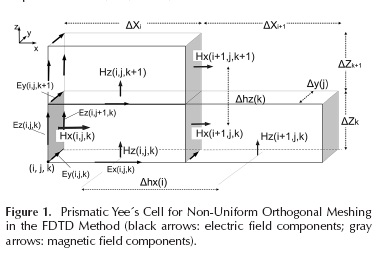
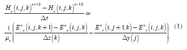
Figure 1 shows three prismatic Yee's cells adjacent to each other, where different edge lengths are considered for the cell located at the (i,j,k) node. It must be also noted that due to the difference between cell edge lengths for each direction 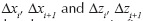the distances Δh_x and Δh_z between the electromagnetic field components will also be variable for each direction. The electric and magnetic field time-updating equations can be found as presented in (Yee, 1966), but taking into account the variable location of the edge centers, the variable cell edge length and the distances between the cell side centers. For illustration, the central difference formulation for a non-uniform cell applied to the x-component of the magnetic field shown in Figure 1 is:

Several techniques can be proposed in order to automatically generate the mesh grid for the computational domain. In (Yang & Chen, 1999) a technique based on the use of a constant growth rate allowed the generation of a mesh pattern within a defined interval. This paper formulates a general algorithm for an arbitrary growth rate function within the interval, which will be referred to as the spacing function. An example for constant growth rate is also presented.

Automatic meshing algorithm for the FDTD method

The strategy proposed in order to impose a non-uniform mesh in a 3D problem space is to use finer mesh nearby elements, such as thin-wires, sources, lumped loads, etc., and a coarser mesh for the rest of free-space intervals in the computational domain.

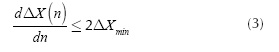
The main objective of the non-uniform meshing algorithm is to find the spatial coordinates within a determined space interval when a spacing function is defined. Consider a closed interval [X_min, X_max] where a non-uniform mesh will be constructed. There are two restrictions that must be imposed to the spacing function in order to guarantee the convergence criteria of the FDTD method. First, the derivative of the spacing function cannot be higher than 2. This means that the maximum length variation between two consecutive cell edges must be twice as maximum in order to avoid significant errors mainly due to the dispersion produced by the non-uniform grid (Svigelj, 1995; Taflove & Hagness, 2005). In second place, the coordinates of the mesh grid must be the cumulative sum of each of the spaces defined by the spacing function.

In order to express these two restrictions in a mathematical form, let ΔX(n) be the desired spacing function with n = 0,1,.... N, where N is the total number of discrete points within the interval. Additionally, let e ΔX_min and ΔX_max be the minimum and maximum spacing lengths, respectively, in order to be used within the interval and be defined as input parameters depending on the dimensions of the geometry to be represented. It must be taken into account that in order to obtain more accurate solutions, the maximum spacing size ΔX_max must satisfy the electrically short criteria by means of which its value must be less than λ_min/10 or λ_min/15, where ?min is the minimal wave-length corresponding to the upper frequency band component of the excitation source (Taflove & Hagness, 2005). The first value of the spacing function must be imposed to be ΔX(0) = ΔX_max in order to include the minimum spacing value in the mesh.

The minimum spacing length ΔX_min selection will determine the time-step value in order to guarantee numerical stability as shown in Equation (2).

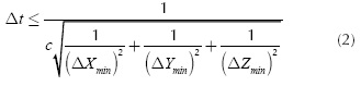
where c is the speed of propagation of the electromagnetic wave in the media (Taflove & Hagness, 2005). It is worth noting that the time-step value is usually chosen as a percentage of the maximum value specified in Equation (2); in this paper we have chosen 0.9 times the maximum time-step value in order to minimize the error due to the space-time discretization. As it has been extensively discussed in (Svigelj, 1995), the error from grid-dispersion due to the non-uniform grid implementation will depend on the time-step value and the variation of the cell side in the non-uniform grid. The latter has been directly included in the second restriction of the algorithm in order to keep the grid dispersion error under 0.1 %, approximately (Svigelj, 1995).

The restrictions mentioned before can be expressed as:

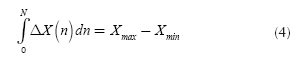
The inclusion of the spacing function into Equations (3) and (4) leads to an equations system whose unknowns are the total number of discrete points N and the maximum spacing length ΔX_max.

Figure 2 depicts a general spacing function defined by N discrete points and the resultant coordinate points that satisfy Equation (4) within the closed interval [X_min X_max].

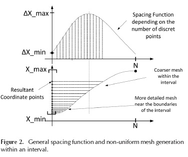
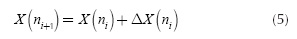
As it can be seen in Figure 2, the spacing function has been proposed in this case to have the minimum spacing length at the interval ends and a larger spacing within it. Once the spacing function has been defined, the mesh coordinates points can be found by evaluating the integral proposed for the second restriction in Equation (4). A recursive scheme for the evaluation of the coordinate points can be found by a first-order backward approach given by:

In order to show the usage of the proposed algorithm, consider a spacing function defined by a sinusoidal function defined for the closed interval [X_min X_max], where the minimum spacing value ΔX_min is known:

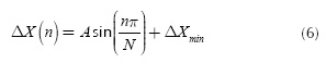
In Equation (6) the unknown variables are: the maximum amplitude of the spacing function A= ΔX_min - Δ X_max the maximum spacing length ΔX_max and the total discrete points for the automatic mesh N. Applying (3) to (6) yields to

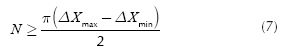
Imposing the second criteria defined in Equation (4) to the spacing function Equation (6) leads to

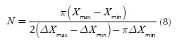
Equations (7) and (8), the maximum spacing length allowed for the interval can be found by:

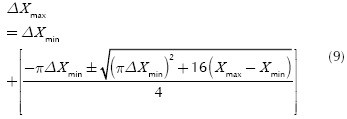
Once Δ X_max has been determined, the spacing function Equation (6) can be used to obtain the coordinate points by means of Equation (5).

Using the approach proposed before, any analytical form of the spacing function can be defined depending on the geometrical features and the variations of the electromagnetic field of a given scenario. Coarser meshes can be defined for slow space-variations of the electromagnetic field and finer ones can be defined for rapid variations or for small detailed structures.

Experimental validation for a two-wire crosstalk set-up

Crosstalk is an effect occurring when two or more transmission lines are close to each other affecting their voltages and currents due to their strong capacitive and inductive coupling. This effect could lead to significant distortion of their own transmitted signals (Ott, 1976; Paul, 2006).

Crosstalk is typically studied in transmission systems used in digital data at high frequencies because the fast wave-fronts of the signals excite the frequency band where the capacitance and inductance coupling effect cannot be neglected and its effect could lead to the corruption of the transmitted data disabling the communication channel.

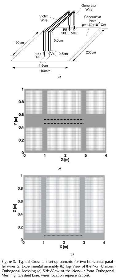
A typical experimental set-up used for evidencing this effect was constructed. The set up was composed by two copper wires with 0.25 mm in radius and a DC resistance per unit length of 84 if/km. Wires were separated a distance of 1.5 cm and each wire was situated at the same height of 5.5 cm from a conductive plate. The plate's resistivity was assumed to be 1.69 x 10^-8ifm.

Generator and victim wires were loaded at each end with a 50 Ω resistor. The generator wire was excited by a ramp voltage source with 50 if of internal resistance. The excitation waveform had a peak value of 20V and 30 ns in wave-front. The experimental assembly is depicted in Figure 3(a).

The simplest spacing-functions that can be defined for the non-uniform mesh are those composed by linear functions whose slopes correspond to the increase rate of the coordinate point values. For the case under study, a piecewise spacing-function was defined for the intervals [X_min X_max] free of wires in the experimental set-up. The spacing-function that was used can be written as:

Where m is the slope of the straight line and the total discrete points in the interval can be calculated by N = 2n1 + n2.

Parameters nl and n2 can be found by imposing the restrictions presented in the previous section and can be calculated by:

Once nl and n2 have been obtained, the non-uniform mesh is completely defined.

The slope m can be set depending on the desired spacing rate. In general m=αΔX_min where α can be set between 0<a<2 in order to consider the minimum and maximum slope, respectively. The α factor can be understood as a decreasing or increasing factor for the spacing rate; α factors lower than the unity implies soft changes on the spacing mesh.

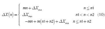
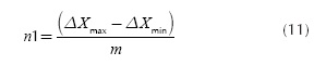
The maximum spacing length was set to be a convenient value for each axis being the maximum one ΔS_max = 50 mm. An attenuator factor α = 0,5mm and a minimum spacing αS = 25 mm were used in order to mesh the problem space. A uniform mesh with the minimum spacing values (ΔX_min, ΔX_min, ΔZ_min) was imposed for regions where the wires and the sources were located. The rest of the problem space regions define the set of closed intervals where the nonuniform automatic-meshing algorithm was applied. Second order Liao's absorbing boundary conditions (Liao, Wong, Yang, & Yuan, 1984) were implemented in order to truncate the computational domain. Figure 3 (b-c) shows the non-uniform mesh obtained for the simulation. Horizontal and vertical wires have been represented using the thin-wire model proposed by (Noda & Yokoyama, 2002) and improved for a smaller radius, as is presented in (Taniguchi, Baba, Nagaoka, & Ametani, 2008).

In order show the advantages of the non-uniform meshing algorithm, the experimental set-up was also simulated by a uniform mesh using a total 1 x 2 x 0.2 m³ space problem with a space cell size length of 2.5mm. For this implementation, CPML absorbing boundary conditions were implemented in order to truncate the problem space (Elshebereni & Demir, 2009).

Using the uniform mesh, a total of 400 x 800 x 80 cells were required to represent the total problem space in the computational domain, in contrast to the proposed non-uniform mesh where a total cell domain of 279 x 181 x 77 were used for a problem space volume of 4 x 1 x 1m³, which means representing 10 times larger problem space dimensions with almost 7 times less computational overhead.

The comparison between the results obtained with uniform mesh and those obtained with the non-uniform mesh is shown in Figure 4.

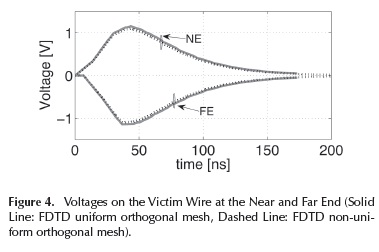
As it can be seen in Figure 4, both results agree very well with the induced voltages on the victim wire. These results validate the usefulness of the non-uniform mesh in the FDTD and the proposed algorithm for the automatic mesh generation.

Figure 5 presents the comparison between those results obtained by using the non-regular orthogonal mesh and the measured voltages on the victim wire.

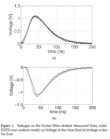
As it may be seen in Figure 5, induced voltages at both ends in the victim wire are well predicted by the theoretical approach. At the near-end a maximum error of about 5 %% was calculated in the mismatched region. At the far-end a lower agreement between both results can be observed, especially for the first time instants leading to up 10 %% in absolute error. This mismatch can be caused by external capacitances and losses in the experimental set-up that were not taken into account for the simulation scenario.

Conclusions

This paper discussed a general algorithm for generating non-uniform orthogonal mesh for the FDTD method. As it was shown, the use of a non-uniform mesh in the FDTD method allows to represent larger problem space dimensions with much less number of Yee's cells. It was also shown that taking advantage of the availability of defining a global minimum spacing, a better representation of the geometries can be performed. An experimental data set was compared with those results theoretically obtained by means of the FDTD method by using a non-regular orthogonal mesh, leading to very good agreements between predicted and measured data.

The proposed algorithm has been formulated in a general mathematical form, where convenient spacing functions can be defined for the problem space discretization allowing the inclusion of small sized objects in the FDTD method and the calculation of detailed variations of the electromagnetic field at desired regions of the computation domain.

References

Elshebereni, A. Z., & Demir, V. (2009). The finite Difference Time Domain Method for Electromagnetics With MATLAB Simulations. (N. S. P. Raleigh, Ed.         [ Links ]).

Jurgens, T. G., Taflove, A., Umashankar, K., & Moore, T. G. (1992). Finite-difference time-domain modeling of curved surfaces. IEEE Transactions on Antennas and Propagation, 40(4). DOI: 10.1109/8.138836.         [ Links ]

Liao, Z. P., Wong, H. L., Yang, B. P., & Yuan, Y. F. (1984). A transmiting boundary for transient wave analyses. Scientia Sinica, XXVII, 1063-1076.         [ Links ]

Noda, T., & Yokoyama, S. (2002). Thin Wire Representation in Finite Difference Time Domain Surge Simulation. IEEE Transactions on Power Delivery, 17(3), 840-847.         [ Links ]

Ott, H. W. (1976). Noise reduction techniques in electronic systems. John Wiley & Sons.         [ Links ]

Paul, C. R. (2006). Introduction to Electromagnetic Compatibility, 2nd Edition. Wiley-IEEE Press.         [ Links ]

Sheen, D. M., Ali, S. M., Abouzahra, M. D., & Kong, J. A. (1990). Application of the three-dimensional finite-difference time-domain method to the analysis of planar microstrip circuits. IEEE Transactions on Microwave Theory and Techniques, 38(7). DOI: 10.1109/22.55775.         [ Links ]

Svigelj, J. A. (1995). Efficient Solution of Maxwell's Equations Using the nonuniform Orthogonal Finite Difference Time Domain Method. University ofIllinois at Urbana-Champaign. University of Illinois at Urbana-Champaign.         [ Links ]

Taflove, A., & Hagness, S. (2005). Computational Electrodynamics: The Finite-Difference Time-Domain Method. (A. House, Ed.         [ Links ]).

Taniguchi, Y., Baba, Y., Nagaoka, N., & Ametani, A. (2008). An improved thin wire representation for FDTD computations. IEEE Transactions on Antennas and Propagation, 56(10), 3248-3252. DOI: 10.1109/TAP.2008.929447.         [ Links ]

Yang, M., & Chen, Y. (1999). An Automatically Adjustable, Non- Uniform, Orthogonal FDTD Mesh Generator. IEEE Antennas and Propagation Magazine, 41(2), 13-19.         [ Links ]

Yee, K. S. (1966). Numerical Solution of Initial Boundary Value Problems Involving Maxwell's Equations in Isotropic Media. Antennas and Propagation, 14, 302 - 307. DOI: 10.1109/TAP.1966.1138693.         [ Links ]