DOI: http://dx.doi.org/10.15446/ing.investig.v36n1.50631

Effects of water inlet configuration in a service reservoir applying CFD modelling

Efecto de la configuración de entrada de agua en un tanque de compensación aplicando modelación CFD

C. Montoya-Pachongo¹, S. Laín-Beatove², P. Torres-Lozada³, C. H. Cruz-Vélez⁴, and J. C. Escobar-Rivera⁵

¹ C. Montoya Pachogo: Sanitary Engineer and Master in Engineering, Universidad del Valle, Colombia. Postgraduate Researcher, University of Leeds, UK. Affiliation: Assistant researcher at Study and Control of Environmental Contamination Research Group (ECCA), Universidad del Valle, Colombia.
Email: cncm@leeds.ac.uk.
² S. Lain Beatove: Physicist, Mathematician and Ph.D. Universidad of Zaragoza, Spain. Dr.-Ing. Habil. Martin Luther University Halle-Wittenberg Germany. Affiliation: Fluid Mechanics Professor, Universidad Autónoma de Occidente, Colombia.
Email: slain@uao.edu.co.
³ P. Torres Lozada: Sanitary Engineer, Universidad del Valle, Colombia. Master and Ph.D, Universidade de São Paulo, Brazil. Affiliation: Permanent Professor at Universidad del Valle, Colombia.
Email: patricia.torres@correounivalle.edu.co.
⁴ C. H. Cruz Vélez: Sanitary Engineer, Universidad del Valle, Colombia. Master, Universidade de São Paulo, Brazil. Affiliation: Associate Professor at Universidad del Valle, Colombia.
Email: camilo.cruz@correounivalle.edu.co.
⁵ C. Escobar Rivera: Sanitary Engineer, Universidad del Valle, Colombia. Master and Ph.D, Universidade de São Paulo, Brazil. Department of Drinking Water Production, EMCALI EICE ESP, Colombia.
Email: jcescobar@emcali.com.co.

How to cite: Montoya-Pachongo, C, Laín-Beatove, S., Torres-Lozada, P., Cruz-Vélez, C., & Escobar-Rivera, J. (2016). Effects of water inlet configuration in a service reservoir applying cfd modelling. Ingeniería e Investigación, 36(1), 31-40. DOI: http://dx.doi.org/10.15446/ing.investig.v36n1.50631.

ABSTRACT

This study investigated the state of a service reservoir of a drinking water distribution network. Numerical simulation was applied to establish its flow pattern, mixing conditions, and free residual chlorine decay. The influence of the change in the water inlet configuration on these characteristics was evaluated. Four scenarios were established with different water level and flow rate as the differences between the first three scenarios. The fourth scenario was evaluated to assess the influence of the inlet configuration, momentum flow and water level on hydrodynamic conditions within the service reservoir. The distribution of four nozzles of 152.4 mm diameter was identified as a viable measure to preserve the water quality in this type of hydraulic structures.

Keywords: Computational fluid dynamics, CFD, free residual chlorine, mixing time, momentum flow, service reservoir, tracer.

RESUMEN

En este estudio se evaluó mediante simulación numérica la influencia del cambio en la configuración de entrada de agua sobre el patrón de flujo, condiciones de mezcla y decaimiento del cloro residual libre en un tanque de compensación de una red de distribución de agua potable. Se establecieron cuatro escenarios, tres presentaron diferencias en el nivel de agua y velocidad de flujo y el cuarto escenario evaluó la influencia de la configuración de entrada, el flujo de momento y nivel del agua sobre las condiciones hidrodinámicas en el tanque de compensación. La distribución de cuatro boquillas de 152,4 mm de diámetro fue identificada como una medida viable para preservar la calidad del agua en este tipo de estructuras hidráulicas.

Palabras clave: Dinámica de fluidos computacional, CFD, cloro residual libre, tiempo de mezcla, flujo de momento, tanque de compensación, trazador.

Received: May 13th 2015 Accepted: January 10th 2016

Introduction

CFD modelling has been widely applied in mechanical engineering and aeronautical industry for being a valuable tool, not only to understand the fluid dynamics but also to reduce associated costs (Lain and Aliod, 2000). This tool has gained acceptance into environmental engineering; specifically in supply water industry, CFD is being applied mainly for assessment and optimization of disinfection processes in reactors commonly located at the end of water treatment train (Angeloudis et al., 2014; Zhang et al., 2014a). For the purpose of this paper, it is necessary to differentiate between disinfection reactors and water storage tanks; the first ones are designed mainly to inactivate potentially harmful microorganisms for public health, where contact time and disinfectant dose are important design and operational variables. Storage tanks refer to the structures located in the distribution network and its functions are to provide water storage volume to attend fire events and absorb water demand peaks. In particular, service reservoirs are storage tanks located in the higher points of the geographic area which additionally compensate the hydraulic pressure in the network, especially when this is supplied by pumping from the water treatment facility, involving fluctuation of the water level.

Traditionally, drinking water storage tanks have been designed and constructed in order to comply with hydraulic functions. During the 1990s, research in water quality inside of storage tanks became of interest and some approaches were developed to find the predominant hydraulic conditions within them in order to infer their effect over water quality. Mainly, those approaches involved operative and/or physical modifications to improve quality of stored water (Lansey and Boulos, 2005). Field experimental studies and modelling are the two basic tools used for research in hydraulic and drinking water quality issues in storage tanks.

Grayman et al. (1996) compared the results of the physical modelling, systems modelling and CFD with experimental data, obtained from a tracer test in a cylindrical tank with simultaneous water inlet and outlet. They found suitable agreement between field data and modelled results. These authors also simulated a tracer test for 33.5 hours and found higher concentrations in the external ring of the tank compared with experimental measurements and also a non-symmetric pattern in its cross section which was not recognized experimentally due to limited sampling points. Additionally, the experimental work identified a significant increase of the tracer in the upper region of the centre of the tank which was not observed in the modelling, likely due to non-consideration of the thermal effects over the flow pattern (Grayman et al., 1996).

Van der Walt (2002) research included CFD simulations of diverse scenarios about free residual chlorine decay in a storage tank. The author concluded that chlorine concentration at the tank outlet is not representative of that of the interior, and established that the minimal permissible limit of residual chlorine should be the criterion to choose a physical modification and/or an operative alternative in a tank to improve the quality of stored water.

Duer (2003) simulated 10 tank configurations by CFD, applying variations in the inlet configuration and water temperature (incoming and stored). The model showed that the studied tank had an inefficient mixing and short circuits due to temperature differences between the stored and incoming water. Mahmood et al. (2005) studied 3 tanks using temperature and residual chlorine measurements and CFD modelling of the tracer injection. From the modelling results, they recommended the use of an inlet with lower diameter in order to increase the momentum and to avoid that the incoming water jet hits the tank walls, improving water mixing. Those modifications were applied to real scale and new experimental data indicated that water showed appropriate mixing.Stamou (2008) studied 9 disinfection tanks. Two configurations, initial geometry and physical modification of the tanks were numerically simulated by CFD. In the initial geometry, flow was characterized by high levels of short circuits, big recirculation regions and low mixing degree; while in the physical modifications, the use of baffles created flow fields with significant volumes of plug flow that reduced short circuits, recirculation zones and increase mixing, resulting in better hydraulic efficiency. Despite the fact that CFD simulations for storage tanks have been performed for constant water level and a specific inlet in most cases, Nordblom (2004) investigated the influence of a denser inflow to a cylindrical tank in transitory mixing processes, using dynamic mesh and grid deformation models to represent fill-and-drain periods in 2 tanks. From numerous simulations under critical conditions of mixing, a range of ratios between water level and tank diameter (H/D) resulting in adequate mixing was recommended. Those simulations demonstrated that the standard k-e turbulence model is sufficient to represent the mixing characteristics in the studied tanks and that CFD modelling could replace more expensive scale model tests and field measurements.

Recently, Zhang et al. (2011) also applied volume-of-fluid (VOF) multiphase analysis and dynamic mesh as strategies for tracking water-level in a rectangular service reservoir, which has inlet and outlet separately and operates with drain cycles or fill-and-drain cycles. Numerical simulations included using the k-e turbulence model and both strategies showed their ability to reproduce the measured water-level variation in the experiments. Hence, the dynamic mesh strategy was applied for further numerical simulations since it significantly saved computational cost. Results showed that the flow in the studied service reservoir presented short-circuiting and poor lateral and vertical mixing. As a result, the chlorine distribution in the reservoir was not uniform, and the lower concentration was found at the recirculation regions. Subsequently, Zhang et al. (2013) evaluated the effect of baffling on the same water reservoir. They concluded that this option is not advisable since it may eventually lead to a diminished effluent chlorine concentration as a result of decreasing flow velocity passing the baffle walls, resulting in an increase of residence time. Finally, the same research team applied dynamic mesh to assess the influence of tank shape on velocity and water age (Zhang et al., 2014b). Based on the last parameter, the authors concluded that a rectangular shape is the best option to be considered for designers when inlet and outlet are separated and located in opposite sites (circular and square shapes were also evaluated). However, this study did not cover thermal stratification, inlet-outlet layout, turnover, and H/D ratio on mixing and age distributions in the CFD simulations (Zhang et al., 2014b).

It is necessary to point out that, to the authors' knowledge, there are not many numerical studies addressing the decay of free residual chlorine in service reservoirs. Most of CFD studies in drinking water distribution systems (DWDS) have focused on comparisons of tracer experimental results with computational simulations. Further application of CFD modelling of the decay of free residual chlorine has been done in chlorine contact chambers, reactors that are characterized by small retention times (few minutes) and higher decay rates in comparison with storage tanks. As a result of that, the application of models representing water variations and free residual chlorine decay in CFD modelling of service reservoirs in DWDS is still required. The works of Nordblom (2004) and Zhang et al. (2011)represent a notable progress in this subject.

Consequently, according to the previous discussion, the objective of this study was to evaluate the influence of the inlet configuration change on flow pattern, mixing conditions and free residual chlorine decay in a service reservoir of a DWDS. This was done by applying CFD in steady state simulations for solving, in first place, the flow pattern with constant water levels, and then this "frozen" flow field was used to separately simulate transient behaviour of tracer transport and chlorine decay. The results of this study allow to conclude that increasing momentum at the inlet improves mixing and promotes flow pattern governed by complete mixing, which is advisable for drinking water reservoirs in order to preserve chlorine concentrations. The authors consider that this study may represent a contribution to the current knowledge of design and operation of drinking water reservoirs in order to preserve water quality in distribution networks.

Methods and Materials

The studied service reservoir, T1, is located in the extreme south of the DWDS of the city of Cali (Col). It is a concrete-made, cylindrical, and ground tank with an internal diameter of 35.12 m, maximal water height of 7.74 m (H/D relation 0.22), and volume equal to 7500 m³. Water to T1 is supplied from a pumping station by a 508 mm diameter cast iron pipeline which is located close to the perimeter and at floor level, working as inlet/outlet. Since T1 compensates pressure in the supplied area, this presents fill-and-drain periods (further details can be found in Montoya et al., 2012).

Simulated scenarios

Considering that T1 operates with fill-and-drain periods according to water demand in the area, the numerical simulation of water level variation requires the inclusion of models that allow the representation of the movement of air-water interphase. For that purpose, models such as VOF or dynamic grid can be used (Nordblom, 2004; Zhang et al., 2011). However, both approaches are very expensive in terms of computational time. In fact, the VOF method was considered by Zhang et al. (2011) and Jaunâtre (2013), but they found it extremely expensive for realistic time period simulations. For instance, Zhang et al. (2011) needed more than 18 days of CPU time to simulate 50 minutes of real time using parallel computing with 8 processors, even using a coarse time step of 0.1 s. Although more economical, the dynamic mesh approach that adds or deletes layers of mesh elements as the simulation progresses still required several days of CPU time to simulate a total real time of around 6 hours, using 10 processors with an extremely large time step of 60 s. For the present study, nor the time or the parallel computer capabilities were available in the research group to afford a full time dependent three-dimensional simulation of the water tank during the required real time of 24 h.

For those reasons, alternative three-dimensional CFD simulations of flow pattern, tracer mixing and free residual chlorine decay were performed with constant water levels, using three operational scenarios based on the experimental results previously discussed by Montoya et al. (2012). In the following, it will be demonstrated that this approach allows to extract practical recommendations which are relevant for the improvement of design and operation of water service reservoirs. Because the physical configuration of the tank and particularly the water inlet plays an essential role in water mixing, a fourth scenario was evaluated in T1. The new scenario involved changing the inlet to four nozzles of 152.4 mm diameter to increase momentum; this was positioned 50 cm above tank bottom and distributed by quadrants, keeping the same water level and flow conditions of scenario 1. Table 1 presents the characteristics of each scenario.

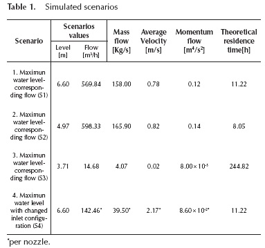
Scenario 4 was defined based on the results of Tian and Roberts (2008), who evaluated 24 tank combinations (cylindrical, standpipe, and rectangular), scale-built with different inlet configurations, conducting tracer tests. The authors found that mixing time decreased by 40 %, using four vertical nozzles as water inlet. Therefore, flow pattern, tracer mixing and chlorine decay simulations were performed for these four scenarios.

Computational approach

In this study, the Reynolds-time-averaged Navier-Stokes (RANS) model is employed to simulate the turbulent flow field inside the tank in connection with the standard k-e turbulence model. The employed software was Fluent v. 6.3. Table 2 shows the conservation law equations used in the numerical simulation of T1. In such Table, p and U are the fluid density and dynamic viscosity respectively, V the fluid velocity vector, and p the pressure. Regarding the turbulent variables, k is the turbulent kinetic energy and e its dissipation rate; mt is the effective viscosity, sum of the molecular viscosity and the turbulent or eddy viscosity (proportional to pk²/e); E is the mean strain rate tensor. SM represents the momentum source realized here for the external gravity field. c represents the mass concentration of the species under consideration.

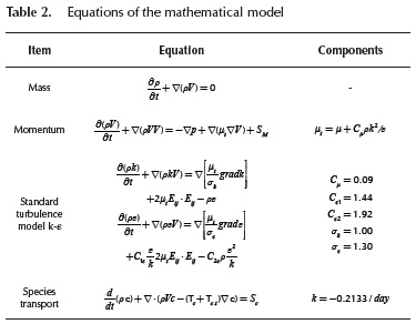
Equations adapted from Fluent (2006)

Tracer was considered as a conservative substance, whereas free residual chlorine in drinking water is a non-conservative substance, since it is a volatile oxidizing agent that also reacts with the organic and inorganic matter present in the bulk water and with the walls that contain it. A chlorine diffusivity in water of 1.4 x 10^-6 Kg/m-s (Poling et al., 2007) was used. The chlorine destruction term was equal to -ρ k C where ρ is the water density, C chlorine concentration and k the chlorine decay constant equal to 0.00000247 s^-1, according to the measurements performed by EMCALI EICE ESP and Universidad del Valle (2007).

The computational mesh used to simulate the four scenarios consisted of a hexahedral multi-block structured mesh, locally refined wherever necessary. Taking into account that T1 does not operate with simultaneous water inlet/outlet, an outlet was defined in the mesh to maintain a constant water level and was located at the bottom of the tank and close to the inlet in order to establish a configuration as close as possible to reality. The difference between meshes of the scenarios was the height that represents each simulated water level (Figure 1).

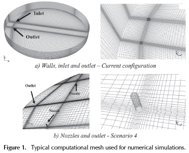
Three meshes with different sizes were initially constructed (with approximately 200,000, 600,000 and 1,000,000 elements) and simulated in steady state for S1. Maximum velocity was the objective variable and its value at the outlet was selected as function of the mesh relative size. As a conclusion of this grid independence study, the difference between the results of the intermediate and fine grids was lower than 1 %. According to the standard analysis of mesh independence verification (Roache, 1998), the intermediate size mesh, of around 600,000 elements, was selected.

Regarding the boundary and initial conditions, mass flow was specified at the inlet and a pressure equal to zero was imposed at the outlet. The walls of the tank were considered as no slip walls and the free surface was stipulated as a zero shear-stress wall. As it was already commented, the standard k-e turbulence model was used to represent the turbulent flow in the numerical modelling of T1 by performing steady state simulations for first solving the flow pattern. Then, transient simulations for tracer transport and chlorine decay from this "frozen" flow field were performed. The discretization approach for the spatial derivatives was of second order. The convergence criterion for the maximal residual of all the variables was 10^-5. The mass flow at the outlet was also monitored to determine when the mass balance was reached. Normalised tracer value was simulated with a value equal to 1 at the inlet during the injection, equal to 0 once this finished, and initially equal to 0 inside of the tank; the injection was performed during a time equal to two times the theoretical residence time (T) for each scenario.

For chlorine, the required time to decrease concentration from 0.92 mg/L to 0.30 mg/L was identified. The initial chlorine concentration was taken as 0.92 mg/L, equal to the average value found in field measurements in the centre of the tank during filling cycles (Montoya et al., 2012). The value of 0.3 mg/L is the permissible minimum value of Colombian regulation (Res. 2115 de 2007 from Ministerio de la Protección Social and Ministerio de Ambiente, Vivienda y Desarrollo Territorial). The numerical simulations were run by employing Fluent 6.3 software in a computer with a processor AMD Phenom (tm) 9750 Quad-Core 2399 MHz, RAM memory of 3.3 GB, using a time step of 10 s for the unsteady simulations (tracer mixing and free residual chlorine). This time step was determined after a sensitivity study, as it was done with the mesh size, testing several time steps (i.e. 20, 10, and 5 sec), finding that velocity values for 5 and 10 sec were similar with a difference lower than 5 %. The simulations to determine the flow pattern in each scenario lasted 2-3 days; those of tracer mixing lasted 2-4 weeks, and those of chlorine decay lasted 4-7 weeks. The longest periods for simulations in unsteady state corresponded to those of S3, that with a lower mass flow.

Data analysis

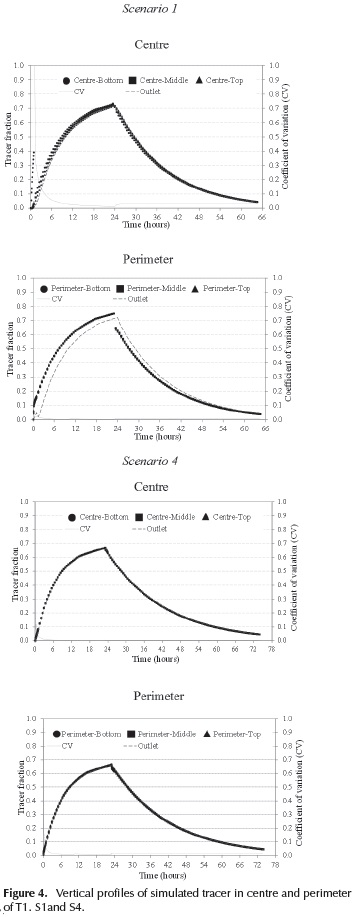
It is known that stagnant zones in hydraulic structures are characterized for close-to-zero velocities, in which reduction of concentrations of non-conservative substances such as chlorine takes place. Hence, these must be avoided in service reservoirs in order to preserve chlorine concentrations in the entire tank. Therefore, regions with the lowest magnitude of the water velocity module different to zero were identified, creating the respective iso-surfaces, which were then overlapped with the streamlines to verify if they matched the recirculation zones. Regarding the tracer simulation, the time in which 95 % of the total tracer fraction left the reservoir was determined, creating tracer iso-surfaces equal to 4 % and 5 % of tracer fraction. These were overlapped with the streamlines to identify the existence and location of stagnant zones. Moreover, vertical profiles of tracer were estimated according to tracer monitoring at top, middle and bottom points in the axis Z (water level).

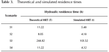
In addition, simulated average residence time (t) was calculated for each scenario according to the distribution of residence times.

Taking into account that the tracer simulations corresponded to a pulse tracer experiment, that inlet and outlet were simulated as separate pipelines, and that the fluid enters only one time to the tank, the accumulated residence time distribution curve F(t) was developed for injection period [F(t) = (Ci/Co), Ci: tracer concentration in t; Co: expected maximum concentration of tracer] (Levenspiel, 1999; Patino et al., 2012). Derivation of F(t) allowed to obtain the residence time distribution curve E(t) and then the area under the curve of t-E(t) was calculated in order to obtain the simulated average residence time (t). Theoretical residence time (T) was calculated from inlet flow rate and water volume (T =V/Q).

Results and Discussion

Flow pattern

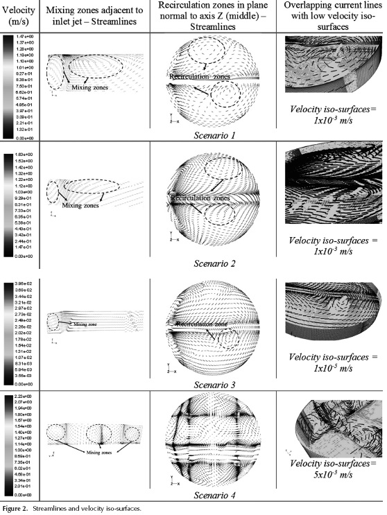
The flow streamlines of scenarios 1-3 show the presence of mixing zones adjacent to the inlet jet, in the water surface as well as in the zone between the wall and the jet (Figure 2). Moreover, there are recirculation zones in the plane located at the mid-height in the tank. The iso-surfaces show that, for S1 and S2, the zones with low velocity (lower than 10^-3 m/s) are scarce. The superposition of those surfaces with the streamlines indicates that at least one corresponds to the stagnation zone, as is illustrated in Figure 2. Streamlines from S4 reflect the presence of mixing zones between jets and between them and walls, in all of the perpendicular planes to the nozzles. In the perpendicular plane to axis Z, at mid-height of water level, those zones are not observed in contrast to the findings with the current inlet configuration. Additionally, the magnitude of the low velocity regions is increased from 10^-3 m/s to 5x10^-3 m/s using four nozzles as water inlet (Figure 2).

Tracer mixing

The tracer contours for each scenario are observed in Figure 3. 100 % of tracer fraction was expected at the end of the injection as an indication of "good" mixing and lower values may indicate poor mixing conditions inside the tank. Figure 3 shows that only tracer fraction between 70 % and 76 % of that expected in S1 and S2 was reached, respectively, while 100 % of the expected fraction was obtained in S3. Considering the duration of the tracer injection in S3, this was sufficient time to allow mixing of the tracer into the entire stored water. However, for the other two, the injection time was insufficient and the short circuits caused a shortcut out for the tracer, indicating that for large water volumes a higher injection time may be required to get the expected tracer concentration with the given current operating conditions.

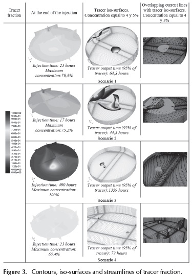
The tracer simulations show that tracer mixing is incomplete into the entire water volume; it enters, hits the water surface and moves from the perimeter towards the centre; because of this, lower concentrations than expected at the end of the injection period are identified in this region. The tracer iso-surfaces reflect the influence of the mass flow in this type of simulations, since the time in which 95 % of the total injected tracer leaves the tank in S2 is lower than S1 (44.5 vs. 63.3 hours) and notoriously lower respect to S3 (1,359 hours). However, the water volumes that still remain inside the tank with tracer fractions of 4 % and 5 % are larger in S1 and S2 than in S3. In addition, the superposition of streamlines with the iso-surfaces of the tracer indicates that the stagnation zones in each scenario correspond to a region of the tank where 4 % and 5 % of the tracer is still remaining. This indicates that under the current conditions the tank has zones in which mixing is inefficient, which may lead to deterioration of the water quality related to significant loss of free residual chlorine. By comparing S1 and S4, the change of the inlet configuration certainly produces the reduction of water volume with tracer fractions of 4 % and 5 %, as observed in Figure 3.

Vertical profiles of the tracer under current conditions indicate that complete mixing was presented after 0.17344.50 h in centre and perimeter of the tank (vertical profiles of S1 and S4 are presented in Figure 4 as an example). This was defined by applying the same criteria of Montoya et al. (2012) to define the mixing time in the experimental evaluation of T1 (coefficient of variation CV < 0.1). However, the tracer contours evidenced that the mentioned mixing is not complete in the whole stored water because there is higher tracer fraction in the perimeter than in the tank centre during the injection, whereas there are zones where 4 % to 5 % of tracer still remains after a 63.3, 44.5, and 1364 hours for S1, S2 and S3, respectively. These results agree with the statements of Jayanti (2001), who emphasized on the interpretation of mixing time, since the calculation of that parameter is based on the arbitrary location of tracer sampling points, resulting in a particular value that would not be equal for the whole water volume. As it can be observed in Figure 4, it is interesting to highlight that the modified inlet configuration (S4) promotes the reduction of the mixing time in 92 % in the tank centre, although a slight increase is present in the perimeter (0.33 h versus 0.50 h, respectively).

Analysis of curves F(t) and E(t)

Under ideal conditions of completely mixed flow, the maximum value expected from the curve F(t) (Figure 5-A) is the unity. However, this was not obtained in the tracer simulations since the tracer period duration (2HRT) was not sufficient to fill the entire water volume with the tracer, as it was previously discussed. As a consequence, S3 presents the maximum value of F(t). According to the exponential-decay shape of the curve E(t) (Figure 5-B), the flow pattern seems to correspond to mixed flow, particularly for S4 and the early sharp peaks indicates shortcuiting between the inlet and outlet. Oscillations of the curve E(t) may represent the presence of certain zones where mixing is not complete (Levenspiel, 1999). In general, analysis of distribution of residence time curves, which focuses on assessment of the tracer variation at a reactor outlet, should be complemented by assessment of the hydraulic pattern inside of the reactor.

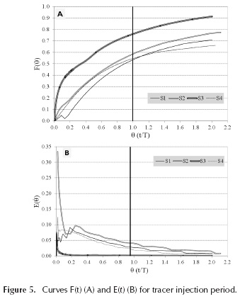
Since curve E(t) is restricted to reactors where the fluid only enters once (close vessel boundary condition) (Levenspiel, 1999), CFD modelling represents a useful tool to analyse the internal hydraulic conditions of service reservoirs where water enters the tank more than one time. Analysis of CV and mixing time seems to be an alternative for these type of tanks as it was explained by Montoya et al. (2012) with experimental tracer data.

The comparison between T vs. t (Table 3) evidences that every scenario presents stagnant zones since the simulated ones are notoriously smaller than the theoretical ones and, as a consequence, the curve E(t) is displaced to the left in relation to T (Levenspiel, 1999). Such stagnant zones in S4 were not identified in the tracer contours (see Figure 3).

Decay of free residual chorine

Chlorine concentrations observed in Figure 6 show that these are influenced mainly by tank filling with fresh water. Such newly injected water drains initial chlorine concentrations since they show a similar pattern than that of tracer fraction, being lower in the tank perimeter, particularly through the zone where the water inlet is located, and higher in the centre. This analysis is also corroborated by comparing chlorine decay in various internal points and at the outlet, which shows that the chorine decay is faster at the points located at one side of the inlet and is slower in the points located next to the outlet, the opposite point to the tank inlet, and in the centre.

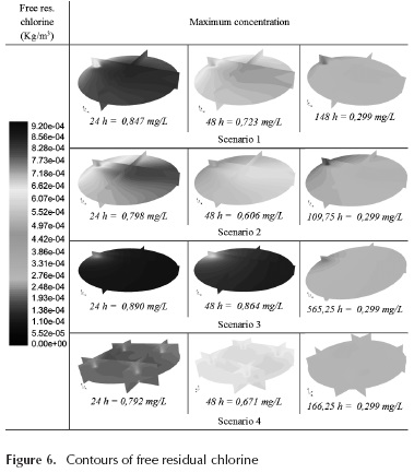
It is important to mention that the chlorine decay is strongly linked to water flow since chlorine simulations correspond to a tank with constant water level; therefore, its exponential adjustment in each scenario results in some correlated decay constants with the respective mass flow. As a result, S2 presents the highest decay constant (0.330 day^-1), followed by S1 and S3 (0.158 day^-1 y 0.085 day^-1, respectively). On the other hand, the water inlet modification of the tank causes that chlorine decays with higher homogeneity in the whole water mass giving a constant decay similar to S1 under current conditions (0.162 day^-1).

Although stagnant zones were identified in the three scenarios under current operating conditions, regions that presented significant reduction of free residual chlorine could not be established as it was identified in the experimental evaluation of T1 (Montoya et al., 2012). This seems to be associated with the adoption of constant water level, since the operation of a service reservoir implies the variation of the water level and the reserve of a water volume for emergency attention, increasing the residence time and easing chlorine decay. In addition, the CFD simulations were performed considering an initial concentration of chlorine equal in the whole water volume.

The results of this study suggest that the current tank characteristics in relation to current momentum flows, water level and inlet configuration do not allow an efficient mixing. Low momentum flows, high water levels, and single and perimeter-located inlet are parameters which combined once negatively affect the hydraulic performance of a service reservoir (dead zones, low water exchange, and poor mixing), leading to low concentrations of free chlorine, sedimentation of suspended particles, and biofilm growth, among others.

Considering that flow variation in T1 depends on water demand in the network and that increasing them in order to obtain higher momentum flows at the inlet represents higher pumping costs, diminishing the maximal levels should be necessary to increase water interchange in current tanks. Additionally, the configuration change at the inlet (diameter reduction and distribution of four nozzles at the tank bottom) shows that the hydrodynamic behaviour notably improves, which is reflected on mixing increase and reduction of the stagnant zones. Different inlet configurations can be tested by CFD modelling for new tanks in order to increase momentum flow magnitude and improve the distribution of the jets to properly mix the stored water volume.

Comparisons with other studies

Van der Walt (2002) studied the water quality inside storage tanks from the perspective of the decrease of free residual chlorine. They evaluated diverse internal configurations for a tank with simultaneous water inlet and outlet, similar to the scenarios considered in the present paper.

Their study concluded that the use of the same behaviour indicators of a tracer for the chlorine decay is not advisable and that plug flow conditions should be established to reduce short circuits and stagnant zones. This can be achieved by means of installation of baffles. The analysis of Stamou (2008) supports the previous conclusions.

In contrast, some other authors claim that, in order to reduce the chlorine decay within the tanks, it is advisable to promote complete mixing because, contrary to disinfection reactors, storage tanks do not have the function of chlorine disinfection. To improve mixing, the energy of inlet jet can be used, avoiding that it hits any surface (Rossman and Grayman, 1999; Jayanti, 2001; Duer, 2003; Grayman et al., 2004). It is worth noting that Zhang et al. (2013) also tested baffling as a strategy to improve mixing and preserve concentration of chlorine in a service reservoir by applying dynamic meshes to represent water-level variation.

Their results evidenced that this is not advisable, since baffles increase water aging and, therefore, effluent chlorine concentrations may be negatively affected. The results obtained in this work, based on CFD simulations of constant water-level scenarios, also support the approach in relation to promote complete mixing in storage tanks.

The previous discussion indicates that more research on this topic is needed and further studies must be developed considering the use of other turbulence models, other inlet configurations, and representation of water level. In this respect, exploiting continuous improvement of CFD codes, numerical methods, and hardware is a requirement for hydraulic and water quality researchers in order to include the numerical representation of water-level variation, using methodologies such as VOF or dynamic meshes.

Conclusions

Inlet configuration in a DWDS service reservoir was evaluated by CFD numerical simulation under constant water-level conditions. It is important to highlight that these type of tanks present variation of water level, and then numerical techniques which allow representation of this feature are recommended in order to validate the model results with experimental data. Therefore, further research into suitable numerical schemes is needed to represent the fluid level variation in reactors which present this behaviour.

This study approach and results allow to present practical recommendations in relation to a desirable mixing pattern, inlet configuration in new service reservoirs, and maximum water level in current tanks. Such recommendations may be useful to water operators and hydraulic designers in order to preserve the drinking water quality in a DWDS.

Hence, the description of flow pattern, mixing conditions, and free residual chlorine was presented. Additionally, the influence of the inlet configuration modification over the mentioned characteristics was evaluated. Stagnant zones were identified in S1, S2 and S3, located mainly in the opposite region to the water inlet, producing high residence times of the tracer. Due to the proximity of the water outlet in relation with the inlet, the presence of short circuits was also determined. Factors such as inlet configuration, flow momentum, and water level are important as they influence the hydrodynamic conditions of a service reservoir. The most critical hydrodynamic conditions were directly related to flow magnitude and stored water volume. They also implied a broad extension of the low velocity zones, high residence time of the tracer, higher volumes with remaining tracer and insufficient tracer mixing in vertical profiles.

The proportional distribution of four nozzles of 152.4 mm led to enhancement of mixing around the jets, higher tracer mixing, reduction in number and dimensions of stagnant zones, and more homogeneous chlorine decay in the water volume. Such modification could represent a feasible measure to preserve water quality inside of service reservoirs. Overall, the results obtained in this study recommend promotion of complete mixing within a drinking water reservoir.

Acknowledgement

The authors would like to acknowledge Colciencias, EMCALI EICE ESP, Universidad del Valle and Universidad Autonoma de Occidente for funding and logistic support.

References

Angeloudis, A., Stoesser, T., Kim, D. & Falconer, R.A. (2014). Predicting the disinfection efficiency range in chlorine contact tanks through a CFD-based approach. Water Research, 60(10), 118-129. DOI: 10.1016/j.watres.2014.04.037.         [ Links ]

Duer, J. M. (2003). Use of CFD to analyze the effects of buoyant inlet jets on mixing standpipes. AWWA. AWWA Annual Conference and Exposition. Anaheim, United States.         [ Links ]

EMCALI EICE ESP and Universidad del Valle. (2007). Investigación y desarrollo de estrategias para reducción del riesgo sanitario en la red de distribución abastecida con agua tratada del río Cauca. Informe final - Tomo I. (Unpublished investigation proyect).Universidad del Valle: Cali.         [ Links ]

Fluent Inc. (2006). Fluent 6.3. User's Cuide. Lebanon: Fluent Inc. Retrieved from http://aerojet.engr.ucdavis.edu/fluen-thelp/pdf/ug/flug.pdf.         [ Links ]

Grayman, M. W., Deininger, A. R., Green, A., Boulos, F. P., Bowcock, W. R. & Godwin, C. C. (1996). Water quality and mixing models for tanks and reservoirs. Journal AWWA, 88(77), 60-73.         [ Links ]

Grayman, M. W., Rossman, A. L., Deininger, D. C., Arnold, N. C. & Smith, F. J. (2004). Mixing and aging of water in distribution system storage facilities. Journal AWWA, 96(9), 70-80.         [ Links ]

Jaunâtre, J. (2013). Numerical simulation of three-dimensional flows in water storage tanks (M.Sc. dissertation). Retrieved from http://lup.lub.lu.se/student-papers/record/4172871. (Report number TVVR-13/5010).         [ Links ]

Jayanti, S. (2001). Hydrodynamics of jet mixing in vessels. Chemical Engineering Science, 56(1), 193-210. DOI: 10.1016/S0009-2509(99)00588-6.         [ Links ]

Lain, S. & Aliod, R. (2000). Study of the Eulerian dispersed phase equations in non-uniform turbulent two-phase flows: Discussion and comparison with experiments. International Journal Heat Fluid Flow, 21(3), 374-380. DOI: 10.1016/S0142-727X(00)00023-0.         [ Links ]

Lansey, K. E. & Boulos, F. P. (2005). Comprehensive handbook on water quality analysis for distributions systems. California: MWH Soft.         [ Links ]

Levenspiel O. (1999). Chemical Reaction Engineering. 3rd edition. New York: John Wiley & Sons.         [ Links ]

Mahmood, F., Pimblett, G. J., Grace, O. G. & Grayman, M. G. (2005). Evaluation of water mixing characteristics in distribution system storage tanks. Journal AWWA, 97(3), 74-88.         [ Links ]

Ministerio de la Protección Social & Ministerio de Ambiente, Vivienda y Desarrollo Territorial. (2007). Resolución No. 2115 del 22 de junio. Retrieved from http://www.ins.gov.co/tramites-y-servicios/programas-de-calidad/Documents/resolucion%202115%20de%202007,MPS-MAVDT.pdf.         [ Links ]

Montoya, C., Cruz, C.H., Torres, P., Lain, S. & Escobar, J.C. (2012). Evaluación de las condiciones de mezcla y su influencia sobre el cloro residual en tanques de compensación de un sistema de distribución de agua potable. Revista Ingeniería y Ciencia, 8(15), 9-30.         [ Links ]

Nordblom O. (2004). Mixing and stagnation in drinking water storage tanks (Doctoral dissertation), Chalmers University of Technology. (ISBN 91-7291-447-5) (Dr Nordblom sent his thesis by post to Carolina Montoya-Pachongo).         [ Links ]

Patiño, P., Cruz, C., Torres, P. & Lain, S. (2012). Hydrodynamic evaluation of a hydraulic clarifier through hydraulic behaviour indicators and simplified flow models. Ingeniería e Investigación, 32(1), 77-82.         [ Links ]

Poling, E. B., Thomson, H. G., Friend, G. D., Rowley, L. R. & Vincent, W. W. (2007). Physical and Chemical Data. In D. W. Green & R. H. Perry (Eds.) Perry's chemical engineers' handbook. New York: Mc Graw Hill.         [ Links ]

Roache, P. J. (1998). Verification and validation in computational science and engineering. Albuquerque: Hermosa Publishers.         [ Links ]

Rossman, A. L. & Grayman, M. W. (1999). Scale-model studies of mixing in drinking water storage tanks. Journal of Environmental Engineering, 125(8), 755-761. DOI: 10.1061/ (asce)0733-9372(1999)125:8(755)        [ Links ]

Stamou, A. (2008). Improving the hydraulic efficiency of water process tanks using CFD models. (2008). Chemical Engineering and Processing: Process Intensification, 47(8), 1 179-1189. DOI: 10.1016/j.cep.2007.02.033.         [ Links ]

Tian, X. & Roberts, P. J. W. (2008). Mixing in water storage tanks. I: no buoyancy effects. Journal of Environmental Engineering, 134(12), 974-985. DOI: /10.1061/ (ASCE) 0733-9372(2008)134:12(986).         [ Links ]

Van der Walt, J. J. (2002). The modelling of water treatment process tanks (Doctoral dissertation). Retrieved from https://ujdigispace.uj.ac.za/handle/10210/471. (Identifier uj: 2269).         [ Links ]

Zhang, J., Lee, H., Khoo, B., Teo, C., Haja, N. & Peng, K. (2011). Modelling and simulations of flow pattern, chlorine concentration, and mean age distributions in potable water service reservoir of Singapore. Journal of Environmental Engineering, 137(7), 575-584. DOI: 10.1061/ (ASCE) EE.1943-7870.0000359.         [ Links ]

Zhang, J., Khoo, B., Lee, H., Teo, C., Haja, N. & Peng, K. (2013). Numerical simulation and assessment of the effects of operation and baffling on a potable water service reservoir. Journal of Environmental Engineering, 139(3), 341-348. DOI: 10.1061/ (ASCE) EE.1943-7870.0000629.         [ Links ]

Zhang, J., Tejada-Martinez, A.E., Zhang, Q. (2014a). Developments in computational fluid dynamics-based modeling for disinfection technologies over the last two decades: A review. Journal Environmental Modelling & Software, 58(8), 71-85. DOI: 10.1016/j.envsoft.2014.04.003.         [ Links ]

Zhang, J., Lee, H., Khoo, B., Peng, K., Zhong, L., Khang C. & Ba, T. (2014b). Shape effect on mixing and age distributions in service reservoirs. Journal AWWA, 106(11), E481-E491. DOI: 10.5942/jawwa.2014.106.0094.         [ Links ]