


Serviços Personalizados
Journal
Artigo
 Inglês (pdf)
 Artigo em XML
 Referências do artigo
 Enviar este artigo por email
Indicadores
-
 Citado por SciELO
 -
 Acessos
Links relacionados
-
 Citado por Google
 -
 Similares em
SciELO
Similares em
SciELO -
 Similares em Google
Compartilhar

 Permalink
Ingeniería e Investigación
versão impressa ISSN 0120-5609
Ing. Investig. vol.36 no.1 Bogotá jan./jun. 2016
https://doi.org/10.15446/ing.investig.v36n1.52810
DOI: http://dx.doi.org/10.15446/ing.investig.v36n1.52810
Isotropic damage model and serial/parallel mix theory applied to nonlinear analysis of ferrocement thin walls. Experimental and numerical analysis
Modelo de daño isótropo y teoría de mezclas serie/paralelo aplicados al análisis no lineal de muros delgados de ferrocemento. Análisis experimental y numérico
Jairo A. Paredes1, Daniel Bedoya-Ruiz2, and Jorge E. Hurtado3
1 Jairo A. Paredes: Civil Engineer, Universidad del Cauca (Popayán). Ph.D. Structural análisis, Polytechnic University of Catalunya, Spain. Affiliation: Associate Prof. Universidad Nacional de Colombia (Manizales).
Email: japaredesl@unal.edu.co.
2 Daniel Bedoya Ruiz: Civil Engineer, Universidad Nacional de Colombia (Medellín). Ph.D. Seismic engineering and structural dynamics, Polytechnic University of Catalunya, Spain. Affiliation:Titular Prof. Universidad Nacional de Colombia (Manizales).
Email: dabedoyar@unal.edu.co.
3 Jorge E. Hurtado: Civil Engineer, Universidad Nacional de Colombia (Manizales). Ph.D. Civil Engineering, Polytechnic University of Catalunya, Spain. Affiliation: Titular Prof. Universidad Nacional de Colombia (Manizales).
Email: jehurtadog@unal.edu.co.
How to cite: Paredes, Jairo. A., Bedoya-Ruiz, Daniel., & Hurtado, Jorge. E. (2016). Isotropic damage model and serial/parallel mix theory applied to nonlinear analysis of ferrocement thin walls. Experimental and numerical analysis. Ingeniería e Investigación, 36(1), 41-51. DOI: http://dx.doi.org/10.15446/ing.investig.v36n1.52810.
ABSTRACT
Ferrocement thin walls are the structural elements that comprise the earthquake resistant system of dwellings built with this material. This article presents the results drawn from an experimental campaign carried out over full-scale precast ferrocement thin walls that were assessed under lateral static loading conditions. The tests allowed the identification of structural parameters and the evaluation of the performance of the walls under static loading conditions. Additionally, an isotropic damage model for modelling the mortar was applied, as well as the classic elasto-plastic theory for modelling the meshes and reinforcing bars. The ferrocement is considered as a composite material, thus the serial/parallel mix theory is used for modelling its mechanical behavior. In this work a methodology for the numerical analysis that allows modeling the nonlinear behavior exhibited by ferrocement walls under static loading conditions, as well as their potential use in earthquake resistant design, is proposed.
Keywords: Precast ferrocement walls, cyclic loading, ductility, Bouc-Wen-Baber-Noori model, earthquake resistant design.
RESUMEN
Los muros de ferrocemento de pared delgada son el elemento estructural principal que compone el sistema de resistencia sísmica de las viviendas de ferrocemento. En este artículo se presentan los resultados de una campaña experimental realizada sobre muros prefabricados de pared delgada de ferrocemento construidos a escala real 1:1, los cuales fueron probados bajo carga estática lateral. Estos ensayos permitieron identificar parámetros estructurales y evaluar la capacidad y el desempeño de los muros bajo carga estática. Adicionalmente, se aplicó el modelo de daño isótropo para la modelación del mortero y la teoría de elasto-plasticidad clásica para la modelación de las barras y la malla de refuerzo. El Ferrocemento se puede considerar como un material compuesto y por lo tanto se utilizó la teoría de mezclas serie/paralelo para modelar su comportamiento mecánico. Así, se planteó una metodología para el análisis numérico no lineal que permite modelar el comportamiento no lineal exhibido por los muros de ferrocemento bajo este tipo de cargas y su potencial uso en el diseño de muros de ferrocemento.
Palabras clave: Muros prefabricados de ferrocemento, carga cíclica, ductilidad, modelo de Bouc-Wen-Baber-Noori, diseño sismo-resistente.
Received: August 31st 2015 Accepted: February 24th 2016
Introduction
The seismic demand determines the material and type of the structural systems to use in housing construction. The presence of earthquakes encourages us to research at innovative systems with better both cost-effectiveness ratio and seismic performance than current systems. Ferrocement-based structural systems are innovative materials with promising applications that have demonstrated high resistance (Wainshtok-Rivas, 1994, 2004; Naaman, 2000; Bedoya-Ruiz, 1998, 2002, 2005; Bedoya-Ruiz et al., 2015), low seismic fragility (Bedoya-Ruiz et al., 2010, 2014 2015), low cost-effectiveness relation, and environmental sustainability (Bedoya-Ruiz, 2011). These systems usually comprise precast thin walls, which are assembled in different configurations according to the constructive system of the dwelling (Naaman, 2000; Castro, 1979; Gokhale, 1983; Olvera, 1998; Wainshtok-Rivas, 1994; Abdullah, 1995; Machado, 1998, Bedoya-Ruiz et al., 2015). The precast ferrocement thin walls give lateral resistance and axial load capacity to the dwellings. This article presents the results drawn from an experimental and theoretical investigation which aims to evaluate the behavior of precast ferrocement thin walls subjected to static loading conditions; we propose a nonlinear numerical model based on an isotropic damage model and the serial/parallel mix theory.
Test specimens
Several ferrocement thin walls were built and tested as depicted below.
Description of the materials
Each wall was constructed using mortar, wire mesh and steel bars. The mortar was made with Portland cement type I (CEM I), sand commonly used in the production of reinforced concrete, water and superplasticizer using the following proportions by weight: sand-cement ratio 1:2, water-cement ratio 0.40, superplasticizer 1 % of cement weight. The superplasticizer was used in order to improve the workability and penetrability of the mortar through the meshes. The reinforcement distributed in the cementitious matrix consisted of six hexagonal mesh layers with an opening of 31.75 mm (this mesh was placed longitudinally); and two #2 bars at the ends of the wall. The specific surface of the reinforcement was 0.0314 mm2/mm3 and its volume fraction was 0.39 %.
The compressive strength of the mortar (f 'cm) after 28 days was 33 MPa, the Young modulus (Ec) of the composite was 11050 MPa; the yield resistance (σry) of the hexagonal mesh was 282 MPa, and its Young modulus (Er) was 81 GPa. Finally, the yield resistance of the #2 bars was 420 MPa.
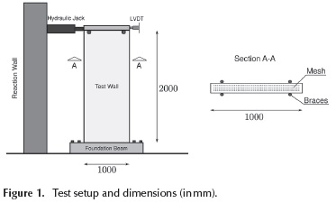
Test setup and load history
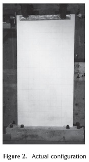
The geometry of each of the specimens is sketched in Figure 1; an overview of the test set up is shown in Figure 2.
Lateral static load test
Ferrocement thin walls are designed not only to resist axial loads, but also forces induced by earthquakes. In the case of walls parallel to the seismic motion, the walls must withstand shear forces generated by the earthquake. In order to compute the strength to lateral static loads, three walls were tested. Figure 1 shows an overview of the test set up.
The walls were anchored to reinforced concrete foundation beams in order to provide lateral support. Thereafter, each "wall-foundation beam" system was anchored to a reaction floor with steel screws as illustrated in Figure 2. In order to constrain the walls to in-plane-displacements, lateral bracing was employed. The lateral displacement induced by the hydraulic actuator was measured using LVDTs placed at the top of the walls.
Test results
The results drawn from the tests are summarized in the next section.
Static load capacity
Figure 3 shows the load vs. lateral displacement curve of the thin ferrocement walls under static loading conditions. Initially, the predominant behaviour was flexural, but the overall response is given by a combination of different reactions. Figure 3 shows some characteristic states of ferrocement under bending loads. Up to 4.0 kN (branch OA), the walls are working under elastic conditions; there are neither cracks to the naked eye nor structural cracks. We obtained an initial stiffness of 6.27 kN/mm from branch OA. As from 4.0 kN, the first structural crack appears (point A in Figure 3). The load vs. displacement curve loses linearity (branch AB, up to 8.0 kN). From this point the first cracks are generated. With the increase of the lateral load, multiple cracks increase their length and width (branch BC). The yield point of the meshes is not well defined (branch CD). The maximum average load for the ferrocement thin walls was 14.4 kN and it was reached at a displacement of 13.9 mm. The panel failed when the top of the wall reached a maximum horizontal displacement of 17.0 mm. In all cases the measured strength was superior to the theoretical one (12.6 kN) (Naaman, 2000). The shear resistance was 14.4 kN/mm, the secant shear modulus (G') was 8.7 kN/mm and the ductility demand capacity for lateral displacement (μ=Δu/Δyield ) was 4.25.
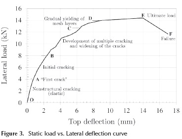
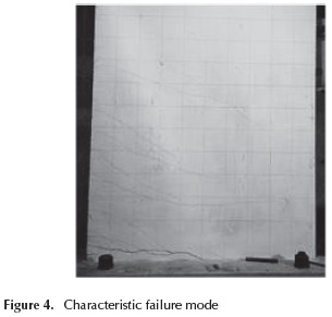
Figure 4. shows a wall after test. Several cracks can be seen in the base of the wall, whose length increased due to increase of the lateral load. It can be observed as well that the walls failed by shear sliding, which is a common failure mode in elements subjected to static loading conditions with a width-height relation less than 2 or 3 (Paulay and Priestley, 1991).
Numerical modelling
Isotropic damage constitutive model
The mechanical behavior of quasi-brittle materials such as concrete, mortar, masonry or rocks is complex. The formation of micro-cracks and the sliding between granular particles generate a highly nonlinear response (Oller, 1988a). This phenomenon is characterized by the influence of the cohesion and friction in the strength of the material, the softening exhibited in the stress-deformation curve, the volumetric expansion (Tao and Phillips, 2005) and, as an obvious consequence, a reduction in the elastic modulus of the material.
Given the broad field of action of these materials (in particular the concrete), several authors have developed different constitutive models that allow us to represent the mechanical behavior of such elements. The Computational Fracture Mechanics (CFM) theory provides bases for these models, mainly for those techniques that are able to simulate the opening and closing of cracks. One of the first applications is due to Hillerborg et al. (1976), who developed a nonlinear fracture model using finite element analysis for modelling the response of reinforced concrete. Other recorded applications include the works performed by Rots et al. (1987), Bazant et al. (1989), among others.
Since 1958, Kachanov (1958) established the bases for damage theory, and they were used to represent the mechanical behavior of different materials. At the beginning, damage modelling was applied to the simulation of dislocation and softening phenomena in steel elements. Simo et al. (1987a, 1987b) proposed the isotropic damage model, and contributions of other authors (Lemaitre (1985), Oliver et al. (1990), Chaboche (1988a, 1988b), Ju (1989), among others) have enabled the constitution of Continuum Damage Mechanics (CDM) as a useful theory for the modelling of quasi-brittle materials.
However, it was only in the early1980's that CDM theory was used for modelling reinforced concrete. Some of those models are based on CDM theory and classic plasticity postulates, e.g. Oller (1988b), Mazars et al. (1989), Lubliner et al. (1989), Jason et al. (2006), Tao et al. (2005), among others.
The continuous damage models are defined from an internal variable that establishes the decrease of both strength and elastic modulus of material; this internal variable can be a scalar or a tensor. The orientation of micro-cracking is not considered for the case of isotropic damage (scalar) (Oliver et al., 1990; Simo et al., 1987a), which ignores the anisotropy effect of the material in the direction of cracking.
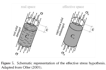
The concept of damage allows us to model the presence of cracks and voids in the material, as well as their evolution (Oller, 2001). In continuum mechanics, this representation can be done by a damage internal variable which relates the effective stress tensor (defined by Kachanov (1958)) and the real stress tensor or Cauchy's tensor σ = (1 - d) σo , where o stands for the Cauchy's stress tensor, which represents the response of the material in the real (damaged) state; σo is the effective stress tensor and it represents the behavior of the material in an undamaged state; and d is the isotropic damage internal variable that measures strength and stiffness degradation of the material. If d=0, it means that the material has not achieved its maximum resistance, hence, the material is undamaged. If the material experiences a total local damage, the internal variable reaches its maximum value: d = 1.
The strain tensor ε is defined as a free variable, and then the effective stress tensor can be computed as σo = Co : ε, where Co is the fourth-order constitutive tensor of the material.
Figure 5 shows a schematic representation of the effective stress hypothesis.
This model agrees with the thermodynamic principles for irreversible, adiabatic and isothermal processes. For an isothermal process the Helmholtz free energy ( ) is defined in terms of the damage variable and the free elastic energy
  . The free elastic energy is a function of the free variable, and is defined as:
 Thermally stable processes must meet the inequality of Clausius-Planck, given by:

where,  is the temporal variation of free energy, defined as:
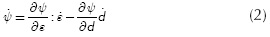
Substituting Equation (2) in (1), the following form of the inequality of Clausius-Planck is obtained:
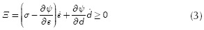
According to Coleman's method (Maugin, 1992), inequality (3) must be satisfied by any temporal variation of the free variable e, therefore, the term in parentheses must be zero, thus obtaining the hyper-elastic constitutive law for the scalar damage constitutive model:
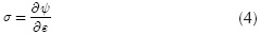
Taking into account the following equation:  we have that the constitutive equation for the isotropic damage model can be written as:
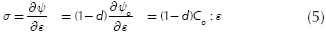
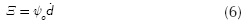
Where σ is the second-order Cauchy's tensor; C0 is the fourth-order elastic constitutive tensor; and is the free energy per unit volume.
The mechanical dissipation can be computed from Equation (3) and the following expression: , obtaining:
For a comprehensive development of the isotropic damage model, the reader is referred to Oller (2001).
Elasto-plasticity constitutive model
In small strain problems, plasticity theory assumes that the total strain is an additive decomposition of the elastic and plastic components ε = ε e + ε p. From the plastic deformation is irreversible, the on-going energetic processes are dissipative and they depend on the trajectory of the stress-strain relation. This relation is given by: σ= C: εe = C: (ε -ε p), where σ is the second-order Cauchy's tensor, and C is the fourth-order elastic tensor. According to the plasticity theory based on continuum mechanics which describes the response of an ideal solid in a macroscopic level, the linear or nonlinear elastic zone is defined by a yield function; whereas that the elasto-plastic region is portrayed by a non-proportional relation between stresses and strains. In this region, the relation between stress increments and strain increments can be positive, zero or negative, depending on the type of elasto-plastic 's hardening, perfect plasticity or softening, respectively. The response is conditioned on the mechanical characteristics of the material.
The behavior on the elastic region is described by Hooke's law; the limit between the elastic and elasto-plastic response is given by a yield function, and the behavior on the elasto-plastic region is described by: (i) the total deformation and its two components (elastic and plastic), (ii) a creep law and (iii) a set of internal variables and its corresponding evolution laws.
The yield function (also known as plastic yield function) is a function of the stress tensor g(σ, q) = 0 where σ is the second-order Cauchy's tensor, and q is a set of internal variables. The plastic yield function is a surface in the stress space covering the elastic zone, which expands or shrinks depending on the plastic behavior of the material (hardening or softening).
The total strain change decomposition has served as a criterion to establish differences among current plasticity theories. For instance, the Levi-von Mises theory states that the total strain increment is equal to the plastic deformation increment  , whereas that Prandtl-Reus theory assures that the total deformation increment is the addition of the elastic strain increment and the plastic strain increment
  ; thus, the relation between stress increments and strain increments is given by:
 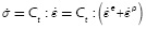 ), where Ct is the fourth-order elasto-plastic tangent tensor.
In small deformations, plasticity theory agrees with Prandtl-Reus hypothesis. Therefore, the plastic strain represents the fundamental internal variable and its evolution is defined by the following creep law:
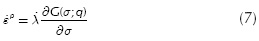
Where G = (σ;q) is the potential creep and  is a nonnegative scalar known as plastic consistency parameter.
When the potential creep is considered equal to the plastic yield function G = (σ;q)  g(σ;q), is said that the creep law is associated. Kuhn-Tucker equations: = 0; g(σ;q) ≤ 0 and g(σ;q)= 0 provide simultaneous conditions that meet Prager's plastic consistency postulate c(σ;q) = 0, and the loading/unloading conditions.
In the present research, each reinforcing bar is represented by an associated elasto-plastic rule. The elastic domain boundary  (σ-,q) = 0 is established through von Mises' yield function; in the case of plastic domain we used an associated creep law according to Prandtl-Reus hypothesis (Oller, 1991); we considered a perfect elasto-plastic response, i.e., it is not necessary the definition of internal variables associated to hardening/softening (William, 2001).
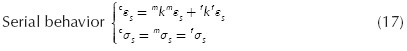
Serial/parallel mix theory
It is very important to determine the physical and mechanical parameters of the ferrocement that will be included within the finite element model. In order to give a proper definition of those parameters, it is necessary to draw upon composite materials theory. Composite materials comprise a matrix that lodges one or several fibres. Ferrocement belongs to this group, because the mortar is the matrix and the meshes are grouped according to their orientation (longitudinal or transversal), and they comprise the fibres.
The definition of mechanical parameters of composite materials has evolved from the classic mix theory to the serial/parallel mix theory in recent years. In classic mix theory, the parameters of the materials are computed from a weighted average according to their volumetric participation. On the other hand, serial/parallel mix theory takes into account fibre orientation as well as loads direction. Throughout this work we applied the serial/parallel mix theory proposed by Rastellini (2006) and implemented by Martinez (2008).
Serial and parallel definition of stress and strain tensors
Serial/parallel mix theory states that the behavior of the materials is parallel in the direction of each fibre, while the behavior is serial on the other directions. In order to take into account this double condition, it is necessary to divide the stress and strain tensors of each component material into their serial and parallel direction.
If we define e1 as the direction vector that determines the parallel behavior, the projection tensor in the parallel direction can be defined as the dyadic product of the unit vector, i.e. Np= e1  e1 , and the fourth-order projection tensor in the parallel direction is defined as: Pp= Np Np . The fourth order projection tensor in the serial direction can be evaluated as the complement of the tensor in the parallel direction, i.e. Ps = l - Np. These fourth-order projection tensors let us divide the strain tensor ε into its parallel and serial components, εp and εs respectively, as follows:


Numerical model hypothesis
The numerical model used to obtain the composite material stress-strain relation based on serial/parallel behavior of its components follows the hypothesis presented below:
-
All materials have the same deformation in the parallel direction (iso-strain condition).
-
All materials undergo the same stresses in the serial direction (iso-stress condition).
-
The contribution of each component materials to the response of the composite is proportional to their volume within the composite.
-
Each component is distributed homogenously within the composite
-
All materials are perfectly bonded.
Constitutive equations of the materials
The behavior of each of material within the composite can be described from their constitutive equations. Reinforced concrete follows a damage constitutive law, and the reinforcing steel is represented by classic plasticity postulates. For these cases, the relation between stress and strain can be written as:


Where kσ is the stress tensor of material k within the composite; kC0 is the respective constitutive tensor; kε and kε p- are the total strain tensor and the plastic strain tensor respectively, and d is the internal variable of the isotropic damage model.
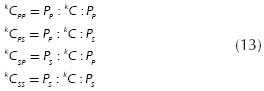
Equations (10) and (11) can be rewritten taking into account the decomposition of the tensors into their serial and parallel components as follows:
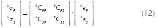
The constitutive tensor of each simple material, represented by superscript k, has been divided into four components according to their participation. Thus, for example, component kCpp is the part of the constitutive tensor which contributes to the parallel behavior; component kCSS is the part whose behavior is completely serial; components kCps and kCSP comprise terms of the constitutive tensor which have serial and parallel behavior combined.
The decomposition of each tensor for each simple material is defined by the double contraction of fourth-order projection tensors and the constitutive tensor, as follows:
Given that both, the matrix material and the fibres, will have a common fourth-order projection tensor, the constitutive tensor of the composite material is determined as a function of the volumetric participation of each simple material, as follows:
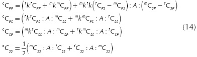
where superscripts c, m and f represent different materials: composite, matrix and fibre respectively. The parameters fk and mk stand for the volumetric participation of each simple material, fibre and matrix respectively.
Equations of equilibrium and compatibility
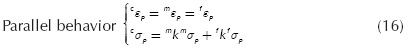
The equations that specify stress equilibrium and establish strain compatibility of the composite are defined from the analysis of the hypothesis presented above. The serial/ parallel mix theory is designed for composite materials with two components: fibre and matrix. With this approach, the relations for both materials in the parallel and serial directions are given by:
Numerical implementation of serial/parallel mix theory
Given that mix theory is a set of constitutive equations, its implementation within a finite element code should be at a constitutive level, i.e., if the input variable is the composite strain tensor cε at a time instant t+Δt, then the algorithm must compute the stress-strain relation of the composite in accordance with the equilibrium and compatibility equations (Equations (16) and (17)); the algorithm should return the composite stress tensor cσ.
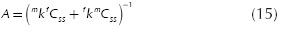
The first step is to divide the strain tensor into its serial and parallel components so as to compute the deformations of the materials (fibre and matrix). After that, we have that the strain parallel component is the same for both materials as indicated by Equation (16). On the other hand, an initial guess must be supplied for the strain serial component of one of the materials; if this prediction is made over the matrix material, then the increase on the expected deformations can be computed as:

where A is defined by Equation (15) and 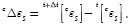
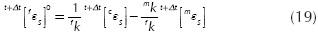
With this first approximation of the matrix serial deformation, we can compute from Equation (17) the fibre strain tensor:
After the serial deformations of both materials have been computed, they must be assembled in conjunction with the parallel components so as to get the strain tensor of each material. At this point, the constitutive equations of each material (Equations (10) and (11)) should be used independently in order to compute the stress tensor and to update the internal variables. The stress serial components for the fibre and the matrix material must meet the equilibrium equation (Equation (17)) within a prescribed threshold, i.e.:

Where, Δσs is the residual stress. If Equation (20) is not verified, then the initial guess for the strain serial component should be corrected using a Newton-Raphson scheme. In this case, the Jacobian is computed as (Rastellini, 2006):
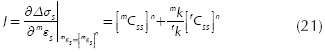
where n is the number of iterations. Once the Jacobian has been determined, the initial guess for the strain serial component of the matrix material is corrected as follows:
In order to obtain a quadratic convergence within the serial/ parallel mix theory, we must use the tangent constitutive tensors of the fibre and the matrix material for computing the Jacobian matrix. Depending on the constitutive equation used for each material, it may be possible that there is not an analytic expression for the tangent constitutive tensor.
This problem was solved by Martinez (2008) and the solution has been implemented within the PLCD routine (Oller et al., 2010), which is a robust derivation algorithm based on perturbations.
Design of composite materials
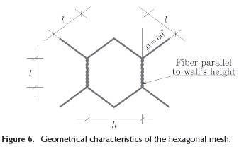
Ferrocement is a composite material made of a mortar matrix as well as hexagonal meshes and reinforcing bars which comprise the fibres. Figure 6 shows the geometry of the reinforcing hexagonal mesh; in this example, the hexagonal mesh is placed longitudinally so each hexagon has two aligned fibres with respect to the longitudinal wall axis, it has two fibres at +60° and other two fibres at -60° with respect to the longitudinal wall axis.
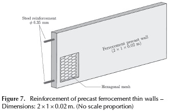
Moreover, each wall has two reinforcing bars of diameter 6.35 mm (#2 bars), located at the ends of the wall. Figure 7 shows a scheme of the wall reinforcement.
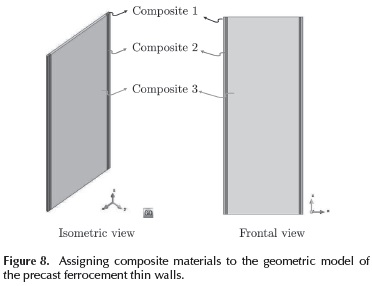
Three composite materials were designed so as to represent the precast ferrocement thin walls:
-
Composite material 1 (MC1): Simple mortar that is assigned to the volumes located at the ends of the wall.
-
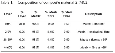
Composite material 2 (MC2): Comprises a mortar matrix, the hexagonal mesh and the reinforcing bars. This material was assigned to vertical volumes where the reinforcing bars are located. The material was designed with 4 layers; Table 1 shows the volumetric participation of each layer as well as the volumetric participation of each material within each layer.
-
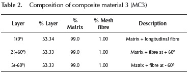
Composite material 3 (MC3 ): This material was used for modelling the matrix and the hexagonal mesh. It was assigned to the central volume of the wall. This material was designed with 3 layers. Table 2 shows the volumetric participation of each layer as well as the volumetric participation of each material within each layer.
The distribution of composite materials within the geometrical model is shown in Figure 8.
Finite element model
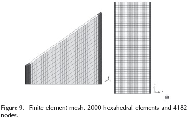
Three different volumes have been defined in order to discretize the precast ferrocement thin walls, and they were assigned to a specific composite material. These volumes were discretized with a mesh of hexahedral elements comprising 2000 elements and 4182 nodes. Each element has 8 integration points and each node has 3 degrees of freedom. Figure 9 shows the finite element mesh employed, the top of the wall is highlighted for illustrative purposes.
Applied loads
The loading process of the precast ferrocement wall comprised two stages: In the first stage we applied a vertical load of 1.46 kN, which simulates the confining load applied at test laboratory; this load was uniformly distributed among the nodes located at the top of the wall. Nodes located at the ends received half the applied load with respect to the intern nodes because those nodes have half afferent area. This stage was executed in one load step. During the second stage, a lateral incremental displacement was applied to the nodes located at the top of the wall; this stage was carried out during 103 load steps. The wall was considered as perfectly fixed at the base.
Numerical results
Response curve
The experimental and numerical response curves are shown in Figure 10. It can be seen that the numerical response curve fits very well the experimental one. The initial slope of the experimental curve is slightly higher than the initial slope of the numerical curve, i.e., the real specimen has higher stiffness than the numerical model. This difference between stiffness values may be due to the support elements that are not included within the numerical model.
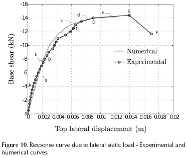
We highlighted some key points of the experimental curve in Figure 3 . and they are shown again in Figure 10. For the numerical curve we highlighted some characteristic points too (a, b, c, d, e), these points will be used to present the numerical results: damage variable, axial strain and stresses.
In the experimental tests, point A corresponds to the first crack appearance, while point a of the numerical curve designates the last point with linear behavior. These two points are close to each other, which could indicate that cracking appearance was captured by the numerical model. The maximum strength measured at laboratory is given by point E, and the maximum strength computed by the numerical model is given by point e. These two values are very close, which shows that the numerical model is able to represent the maximum strength of precast ferrocement thin walls.
Damage evolution
Damage started at the base of the wall in the traction zone. The initial damage appeared at a lateral displacement of 0.0015 m at the top of the wall with an initial value of 0.42907 (point a). The evolution of the damage variable is shown in Figure 11. It can be seen that damage increases in the traction zone and the wall experiences local damages at different points when the top of the wall has reached a lateral displacement of 0.006 m (point c).
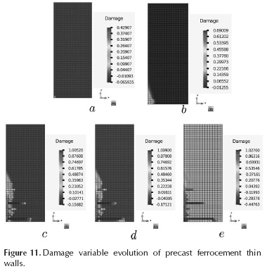
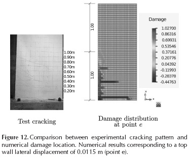
Regions with high values of the damage variable agree with the cracking pattern experienced by the ferrocement walls at laboratory (see Figure 4). The experimental cracking pattern and the damage variables location are shown in Figure 12. The figure on the left shows the state of the wall at the end of the test, the figure on the right correspond to the numerical simulation when the top of the wall has reached a lateral displacement of 0.0115 m (point e). As can be seen, there is a close fit between the experimental cracking zone and the numerical damage location.
Strain evolution
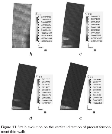
The damage constitutive model that was used for modelling the mortar is based on continuum mechanics. Discontinuity phenomena such cracking formation and their evolution are normally represented by location of deformations.
Frequently, the location of deformations coincides with regions where the damage variable has higher values. The evolution of the vertical strain is shown in Figure 13, and it can be seen that at point b the vertical strain is relatively symmetric, but as the slope of the response curve decreases (point c), two regions with concentrated traction vertical strains come out. Traction strains are 8 times higher than compression deformations. For states corresponding to the final loading stages (points d and e), higher strain values are located at the base of the wall, where the biggest crack was formed.
Stress evolution
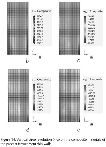
Modelling of composite materials using serial/parallel mix theory allows us to compute the stresses developed on the composite material as well as on each component material. The vertical stress evolution over the three materials is shown in Figure 13 (see Figure 8) defined within the model.
At point b, which is the beginning of damage evolution, we can see that the maximum traction stress (7784.5 kPa) and maximum compression stress (9029.3 kPa) are relatively symmetric; those maximum values are developed by the composite material 2 MC2 (see Figure 8 ) where the reinforcing bars are located.
When the slope of the response curve diminishes (point c), the stress values increase to more than double with respect to point b values and the stress distribution is preserved. The maximum tensile stress for points d and e of the response curve tend to decrease, but keeping the regions with maximum stresses located on MC2 materials, which indicates that the intern flexural moment is developed by the reinforcing bars; additionally, it can be seen that, at point e, regions with MC3 materials (see Figure 8 ) have stress values close to zero, this is due to a high tensile damage at the base (see Figure 12), so the resistance developed by this part of the wall is low.
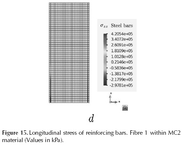
The longitudinal stress distribution over the reinforcing bars (fibre 1 within MC2 material) is shown in Figure 15. It can be seen that the reinforcing bars developed a maximum tensile stress of 420 MPa and a maximum compressive stress of 297 MPa.
The distribution of the principal stress I in both materials, the matrix and the fibres, that comprise MC3 material is shown in Figure 16, where it can be observed that the distribution and magnitude of such stress is similar for the three layers within the matrix (see Table 2), but the magnitude and distribution of the principal stress is different for each layer of the fibres.
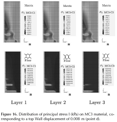
The layer that contains the meshes placed longitudinally experiences high tensile stresses in the regions with higher damage, because the meshes withstand the stresses that the matrix is unable to endure. The layer with fibres at +60° (layer 2, see Table 2) experiences higher stresses than layer 1, probably due to the cinematic loads applied that form a small angle with respect to this layer. The layer with fibres at -60° has the small values of principal stress and it is concentrated at the base of the wall, which coincides with the maximum damage region.
Conclusions
The constitutive isotropic damage model and serial/parallel mix theory have been applied to modeling of ferrocement thin wall subjected to lateral loads. The numerical results fit the experimental ones. It does mean that the ferrocement thin walls can be numerically modelling like a composite material.
The ferrocement has been modeling into several layers. This procedure allows to determine the stresses and strains in each component material. The evolution of isotropic damage variable represents the evolution of cracks in mortar.
Acknowledgements
This investigation has been funded by Universidad Nacional de Colombia under DIMA Grant No. 20301002870: "Estudio y comportamiento sísmico de estructuras de materiales económicos de construcción, tales como el ferrocemento y otros materiales, por medio del análisis experimental y el análisis numérico determinista y estocástico". This support is gratefully acknowledged.
References
Abdullah, A. (1995). Applications of ferrocement as low-cost construction materials in Malaysia. Journal of ferrocement, Vol. 25, No. 2,123-127. [ Links ]
Bazant, Z.P. and Pijaudier-Cabot, G. (1989). Measurement of Characteristic Length of Nonlocal Continuum. Journal of Engineering Mechanics, Vol. 115, 755-767. DOI: 10.1061/(ASCE)0733-9399(1989)1 15:4(755). [ Links ]
Bedoya-Ruiz, D. A. (1998) Diseño sismo resistente de un sistema estructural modular con elementos prefabricados de ferrocemento. (Funpublushed dissertation), Universidad Nacional de Colombia, Medellín. [ Links ]
Bedoya-Ruiz, D.A., Farbiaz, J., Hurtado, J.E., Pujades, L. (2002) Ferrocemento: Un acercamiento al diseño sismo-resistente. Monografías de Ingeniería sísmica. Centro Internacional de Métodos Numéricos (CIMNE). ISBN 8495999-3-4. Spain. [ Links ]
Bedoya-Ruiz, D.A. (2005) Estudio de Resistencia y vulnerabiidad sísmicas de viviendas de bajo costo estructuradas con ferrocemento (Unpublished doctoral dissertation) Universidad Politécnica de Catalunya. Spain. [ Links ]
Bedoya-Ruiz, D.A. Hurtado, J.E., Pujades, L. (2010) Experimental and analytical research on seismic vulnerability of low-cost ferrocement dwelling houses. Structure & Infrastructure Engineering, Vol. 6. No. 1-2, 55-62. DOI: 10.1080/15732470802663789. [ Links ]
Bedoya-Ruiz, D.A. (2011). Experiencias sobre residuos agro-industriales en la construcción de viviendas de ferrocemento (Unpublished dissertation) Universidad Politécnica de Valencia. Spain. [ Links ]
Bedoya-Ruiz D, Ortiz G, Alvarez D.A. (2014) Behavior under cyclic loading of precast ferrocement thin walls: an experimental and analytical research. Revista Ingeniería e Investigación, Vol. 34, No. 1, 29-35. DOI: 10.15446/ing.investig.v34n1.40420. [ Links ]
Bedoya-Ruiz, D., Gilberto A. Ortiz, Diego A. Álvarez and Jorge E. Hurtado. (2015). Modelo dinámico no lineal para evaluar el comportamiento sísmico de viviendas de ferroce-mento. Revista Internacional de Métodos Numéricos para Cálculo y Diseño en Ingeniería. Vol. 31, Issue 3, 139-145. DOI: 10.1016/j.rimni.2014.04.00. [ Links ]
Castro, J. (1979). Application of ferrocement in low-cost housing in Mexico. American Concrete Institute. Vol. 61, 143-146. [ Links ]
Chaboche, J.L. (1988). Continuum Damage Mechanics: Part I- General Concepts. Journal of Applied Mechanics, 55, 5964. DOI: 10.1 1 15/1.3173661. [ Links ]
Chaboche, J.L. (1988). Continuum Damage Mechanics: Part II- Damage Growth, Crack Initiation, and Crack Growth. Journal of Applied Mechanics, 55, 65-72. DOI: 10.1115/1.3173662. [ Links ]
Gokhale, V. G. (1983). System built ferrocement housing. Journal ferrocement. Vol. 15, NO.1, 37-42. [ Links ]
Hillerborg, A., Modéer, M. and Petersson, P.E. (1979). Analysis of crack formation and crack growth in concrete by means of fracture mechanics and finite elements. Cement and Concrete Research, ó, 773-781. DOI: 10.1016/0008-8846(76)90007-7. [ Links ]
Jason, L., Huerta, A. Pijaudier-Cabot, G. and Ghavamian, S. (2006). An elastic plastic damage formulation for concrete: Application to elementary tests and comparison with an isotropic damage model. Computer Methods in Applied Mechanics and Engineering, 195, 7077-7092. DOI: 10.1016/j.cma.2005.04.017. [ Links ]
Ju, J.W. (1989). On energy-based coupled elastoplastic damage theories: Constitutive modeling and computational aspects. International Journal of Solids and Structures, 25, 803-833. DOI: 10.1016/0020-7683(89)90015-2. [ Links ]
Kachanov, L.M. (1958). Time of rupture process under creep conditions. Izvestia Akaademii Nank, 8, 26-31. [ Links ]
Lemaitre, J. (1985). Coupled elasto-plasticity and damage constitutive equations. Computer Methods in Applied Mechanics and Engineering, S1, 31-49. DOI: 10.1016/0045-7825(85)90026-X. [ Links ]
Lubliner, J., Oliver, J., Oller, S. and Oñate, E. (1989). A plastic-damage model for concrete. International Journal of Solids and Structures, 2S, 299-326. DOI: 10.1016/0020-7683(89)90050-4. [ Links ]
Machado Jr., E. F. (1998). Building system for low-cost ferroce-ment housing. Memoirs from Ferrocement ó: Lambot symposium. Proceedings of the sixth international on ferroce-ment. Michigan. Editor: A. E. Naaman. 129-138. [ Links ]
Martinez, X. (2008). Micro mechanical simulation of composite materials using the serial/parallel mixing theory. (Unpublished doctoral dissertation) Universidad Politécnica de Cataluña. Spain. [ Links ]
Maugin, G.A. (1989). The thermodynamics of plasticity and fracture, Cambridge University press. [ Links ]
Mazars, J. and Pijaudier-Cabot, G. (1989). Continuum Damage Theory Application to Concrete. Journal of Engineering Mechanics, 11S, 345-365. DOI: 10.1061/(ASCE)0733-9399(1989)115:2(345). [ Links ]
Naaman, A. E. (2000). Ferrocement and laminated cementitious composites. Techno Press 3000. Michigan. [ Links ]
Oliver, J., Cervera, M., Oller, S. and Lubliner, J. (1990). Isotropic damage models and smeared crack analysis of concrete. In: Proc. 2nd. Int. Conf. on Computer Aided Analysis and Design of Concrete Structures, Zell am See, 945-58. [ Links ]
Oller, S. (1988a). Un modelo de daño continuo para materiales-friccionales.(Unpublished doctoral dissertation), Universidad Politécnica de Cataluña. Spain. [ Links ]
Oller, S. (1988b). Un modelo de daño continuo para materiales-friccionales. (Unpublished doctoral dissertation)Universidad Politécnica de Cataluña. Spain. [ Links ]
Oller, S. (1991). Modelización numérica de Materiales Friccionales, CIMNE. Barcelona. [ Links ]
Oller, S. (2001). Fractura Mecánica. Un enfoque global. CIMNE. Barcelona. [ Links ]
Oller, S., Luccioni, B., Hanganu, A., Car, E., Salomon, O., Neamtu, L., Zalamea, F., Mata, P., Martinez, X., Molina, M., Paredes, J.A. and Otero, F. (2010). Breve Manual de PLCD. Barcelona. [ Links ]
Olvera López, A. (1998). Applications of prefabricated ferrocement housing in Mexico Memoirs from Ferrocement 6: Lambot symposium. Proceedings of the sixth international on ferrocement. Michigan. Editor: A. E. Naaman. 95-108. [ Links ]
Pauly, T., Priestley, M. J. N. (1991). Seismic design of reinforced concrete and masonry buildings. New York: Ed. Jhon Waley and Sons, INC. [ Links ]
Rastellini, F. (2006). Modelización numérica de la no-linealidad constitutiva de laminados compuestos. (unpublished doctoral dissertation), Universidad Politécnica de Cataluña. Spain. [ Links ]
Rots, J.G. and Borst, R.D. (1987). Analysis of Mixed-Mode Fracture in Concrete. Journal of Engineering Mechanics, 113, 1739-1758. DOI: 10.1061/(ASCE)0733-9399(1987)1 13:1 1(1739). [ Links ]
Simo, J.C. and Ju, J.W. Strain- and stress-based continuum damage models-I. (1987a). Formulation. International Journal of Solids and Structures, 23, 821-840. DOI: 10.1016/0020-7683(87)90083-7. [ Links ]
Simo, J.C. and Ju, J.W. (1987b). Strain- and stress-based continuum damage models-II. Computational aspects. International Journal of Solids and Structures, 23, 841-869. DOI: 10.1016/0020-7683(87)90084-9. [ Links ]
Tao, X. and Phillips, D.V. (2005). A simplified isotropic damage model for concrete under bi-axial stress states. Cement and Concrete Composites, 27, 716-726. DOI: 10.1016/j.cemconcomp.2004.09.017. [ Links ]
Wainshtok-Rivas, H. (1994). Low-cost housing built with ferrocement precast elements, Journal of ferrocement, Vol. 24, No. 1, 29-34. [ Links ]
Wainshtok-Rivas, H. (2004). Model seismic resistant ferroce-ment houses. Journal of ferrocement, Vol. 34, No. 2, 363-371. [ Links ]

