DOI: http://dx.doi.org/10.15446/ing.investig.v36n2.52775

Effect of the height of the greenhouse on the plant - climate relationship as a development parameter in mint (Mentha Spicata) crops in Colombia

Efecto de la altura del invernadero en la relación planta - clima como parámetro de desarrollo en cultivos de menta (Mentha Spicata) en Colombia

N. Bustamante¹, J. F. Acuña C², and D. L Valera³

¹ PhD(c) in Agriplasticulture. Affiliation: Commercial and technical advisor, P. Q. A. S. A., Colombia. E-mail: nelson@pqa.com.co.
² PhD in Agricultural mechanization and technology. Affiliation: Associate Professor at Universidad Nacional de Colombia. Colombia. E-mail: jfacunac@unal.edu.co.
³ PhD in Agricultural Engineering. Affiliation: Associate Professor at Universidad de Almería, Spain. E-mail: dvalera@ual.es.

How to cite: Bustamante, N., Acuña, J. F., & Valera, D. L. (2015). Effect of the height of the greenhouse on the plant - climate relationship as a deve­lopment parameter in mint (Mentha Spicata) crops in Colombia. Ingeniería e Investigación, 36(2), 06 - 12. DOI: 10.15446/ing.investig.v36n2.52775.

ABSTRACT

The aim of the study is to evaluate the effect of the height of the greenhouse on climatic conditions generated on a mint crop (Mentha spicata). The tests were conducted in the town of Carmen de Viboral, 40 minutes away from the city of Medellin (6° 05' 09" N and 75° 20' 19" W, 2150 m.a.s.l.). Three greenhouses with the same dimensions were used, changing only the gutter height in 2 m, 2,5 m and 3 m respectively. Temperature and relative humidity measurements were taken every 30 minutes for 3 years, time during which crop production was assessed. Statistical analyses were performed to determine climatic variations caused by the difference in height between the greenhouses, and to determine differences in production levels. The results indicate that, under the study conditions, the greenhouse height directly affects the weather conditions and the mint crop yields.

Keywords: Greenhouses, climate control, environmental control, mint crops.

RESUMEN

El objetivo del estudio es evaluar el efecto que produce la altura del invernadero en las condiciones climáticas generadas sobre un cultivo de menta (Mentha spicata). Los ensayos se realizaron en el municipio del Carmen de Viboral, a 40 minutos de la ciudad de Medellín (6°05'09" N y 75°20'19" W, 2150 m.s.n.m.). Se utilizaron 3 invernaderos de iguales dimensiones, variando solamente su altura de canal de 2 m, 2,5 m y 3 m respectivamente. Se realizaron mediciones de temperatura y humedad relativa cada 30 minutos por 3 años, durante los cuales se evaluó la producción del cultivo. Se realizaron análisis estadísticos para determinar las variaciones climáticas causadas por la diferencia de altura entre los invernaderos, así como para determinar diferencias en los niveles de producción. Los resultados indican que para las condiciones del estudio la altura del invernadero incide directamente en las condiciones climáticas y en los rendimientos del cultivo de menta.

Palabras clave: Invernaderos, control climático, ambiental, cultivos de menta.

Received: August 29th 2015 Accepted: July 8th 2016

Introduction

Changes in the environment exert different pressures on plants and influence the development of each species, resulting in various forms of growth, which should be interpreted as different paths the plants have followed to adapt to a particular environment (Sherry et al., 2007). The biological life cycle changes with the genotype and climatic factors, meaning that plants from the same genotype planted under different weather conditions may have different development stages after the expiry of the same chronological time. Therefore, biological events are used as indicators of the presence or absence of certain environmental factors to draw certain conclusions or make predictions about plant responses (Dahlgren et al., 2007).

Thermal energy is the main environmental factor influencing plant development rate (Lambers et al., 2008). Sadras et al. (2000) defined plant development as a progressive sequence of distinct morphological and physiological states. Variations in environmental conditions alter the evolution of the fundamental metabolic processes, transport of assimilates, growth evolution, leaf expansion dynamics and biomass partition factors (Salisbury and Ross, 2000).

The production of high quality plants is directly affected by light and temperature. These factors are modified by changing the geometry of the greenhouse or cover film type used. The particular geometry directly influences the natural ventilation of the greenhouse, which occurs mainly by the combined action of wind and buoyancy forces (Roy et al,. 2002). The local environment is a determining factor in the growth of plants, and their response to these factors depends on their variety and physiological state. (Quintero et al,. 2014). This paper aims to show on the one hand, that by changing the height of the greenhouse, different climatic conditions inside are generated; and, on the other hand, what is the most appropriate height of greenhouse for growing mint in tropical mountains.

Materials and methods

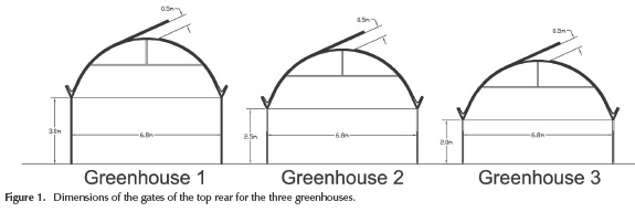
The tests were conducted in the town of Carmen de Viboral, 40 minutes away from Medellin (6° 05' 09" N and 75° 20' 19" W, 2150 m.a.s.l.). 3 metal multi-tunnel greenhouses with 4 bays covering an area of 1523,2 m² each, with the same dimensions and roof slopes, changing only their gutter height at the end of the greenhouse by 2 m, 2,5 m and 3 m respectively, were used (Figure 1).

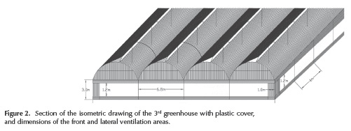
Screens are distributed around the perimeter: two side (1,2 m x 54 m) and two front screens (1,2 m x 25,2 m) are operated manually, which are opened at 6 am and closed again after the end of working hours (4 pm). Each bay with dimensions of 6,8 x 56 m consists of 15 separate frames every 4 m. The structure is clamped with 1/8" galvanized longitudinal and transverse cables duly anchored in the ground (Figure 2).

A production monitoring and data collection of temperature and relative humidity was performed in the three greenhouses, and measurements in the outside of the greenhouses were taken for reference over a period of three years starting on January 5, 2012.

A baseline irrigation, fertilization and spraying program was implemented, so that the overall handling of the three crops in these areas was a constant factor in the study. The spraying was done based on the monitoring carried out in the field, with indications and preventive (not shock) dosages in order not to alter the product. Crop work and weeding was done every two weeks; and hoeing was done every three months.

The temperature and relative humidity were analyzed on the greenhouse throughout the study period, from January 5, 2012, to January 21, 2015. During this period, 2 full cycles of mint (12 cuts per cycle) and the first 4 cuts on the third cycle were measured; for a total of 308 pieces of data for greenhouse production.

Data taken with a multiple linear regression was performed to study the relationship between the two study variables (temperature and humidity) with the response variable (production). A collinearity analysis to study the relationship between the two independent variables (temperature and relative humidity) was made, which helps to interpret the data obtained from the linear regression and the analysis of heteroscedasticity to verify that the variance of the input disturbance variables are not constant. For statistical analysis, the SPSS software was used.

Analysis of results

Mint crop production data

The cultivation of mint has a production cycle of 12 months; the time of study of this work was three years, so the production data are available for a total of 30 cuts for the cycles mentioned above. Table 1 shows the total production obtained per cycle and per greenhouse.

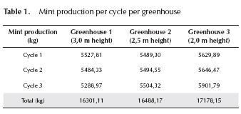
Table 1 shows that most production takes place in the 3^rd greenhouse, with 17178,15 kg of mint produced. This greenhouse has a minimum channel height of 2 m. While for the 1^st and 2^nd greenhouses the production did not differ by more than 1,15 %; if we compare the 1st and the 3^rd greenhouse, we have a difference in production of 5,38 %. This tends to tell us that the best mint productions would take place in a low greenhouse.

Statistical analysis

Linear regression of the mint crop production data

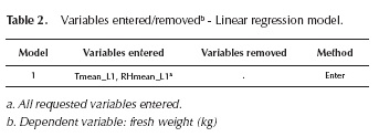
Regression analysis of mint is made depending on temperature and relative humidity as a first step for statistically evaluating the influence of these variables on the response variable, which was the production in kg.

In Table 2 the input variables can be seen in the regression model.

Once the variables are introduced, the regression process with SPSS software is made and the results shown on Table 3 are obtained:

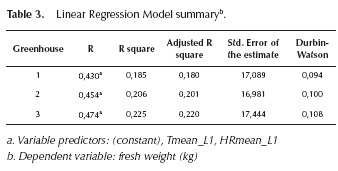
The data shows the existence of a global linear association between the predictor variables and the response variable, considering that the R² was different from 0 in the three greenhouses. Its magnitude suggests the percentage of the variations in the response variable was given by the variations of the predicting variables.

For instance, in the case of the 2^nd greenhouse, the model says that the joint variation of the Tmean and RHmean explain 20,6 °% of the variations in fresh weight obtained. The statistical DW for the 3 cases was lower than 2; allowing the statistical statement that there is a negative autocorrelation between the predicting variables. This coincides with the normal behavior of these two variables where one has higher temperature and lower relative humidity, and vice versa.

In order to evaluate if the regression model is valid globally, an ANOVA variance analysis (Table 4) was performed to verify jointly the explanatory variables or predictors (RH and T), which provide information explaining the response or dependent variable (fresh weight).

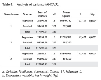
The null hypothesis in this case is that the predictor variables are not linearly related to the dependent variable. For this, the value of the F statistic is compared with the critical value given by the degrees of freedom of the table and a significance level of 5 °%. The critical value and the comparison are calculated internally by the software, expressing the Sig value with a value equal to 0,000. This value indicates that, with a significance level of 5 °%, there is certainly a significant linear relationship between crop production (measured in kg of fresh weight) and the relative humidity and temperature variables of each of the greenhouses.

After verifying the validity of the model, we proceed to calculate regression coefficients as shown in Table 5.

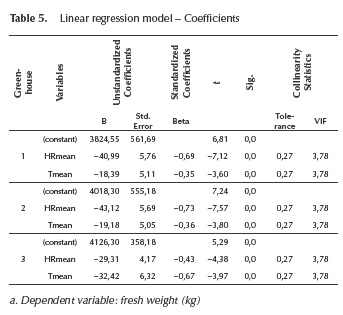
The t test values and their level of significance (Sig) are used to compare the null hypothesis that the respective regression coefficients take a zero value. According to the results, in all cases the null hypothesis is rejected; that is, all the coefficients obtained are relevant to the regression equation. Meanwhile, the values of statistical collinearity show that this feature does not affect the validity of the model, since no values higher than 10 are obtained in the variance inflation factor VIF (Kleinbaum et al., 1988).

Below, the regression equations of the mint crop that forecast the production value according to variations in temperature and relative humidity for each greenhouse are shown.

1^st Greenhouse Equation:

2^nd Greenhouse Equation:

3^rd Greenhouse Equation:

The linear regression procedure comes from the assumptions of normality and homoscedasticity of waste, i.e. the behavior of the differences between the equations predicted and the actual value follows the normal distribution. In order to evaluate this, the normal probability graph shown in Figure 3 is devised.

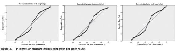
As shown in the charts, in all three cases there is a tendency of the point cloud to align to the diagonal line on the graph, which warns that the normality assumption in the data is true.

Regression collinearity analysis of the mint crop data

The collinearity analysis helps confirm if there is a high ratio of dependent or predictor variables. At once we know that this does happen because of the inverse relationship that occurs between temperature and relative humidity under normal conditions. In order to verify this statistically, a collinearity test is done, the results of which are shown on Table 6.

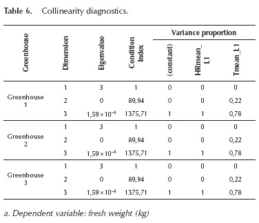
Below are 3 ways to interpret the above table to determine the presence of collinearity (Brown et al., 2005)

1. When most of the eigenvalues are close to zero.
2. When the condition indexes are greater than 30.
3. For higher indexes, when two or more factors have a larger proportion to the variance.

These three conditions are met for all greenhouses, meaning that it is confirmed that the data obtained from measurements stored are consistent with the normal behavior of these two variables.

Correlations of the mint crop data

On the assumption of normality in the data, at the beginning, a Pearson correlation (Table 7) is done, which is performed when the data follow a normal distribution. Additionally, two correlations are done: the Kendall Tau_b (Table 8) and the Spearman Tau_b (Table 9), which are used as alternatives to Pearson when the studied variables violate the assumption of normality.

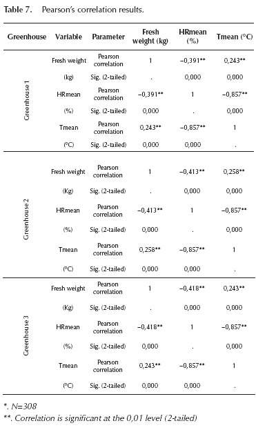
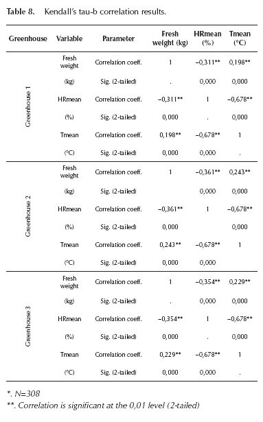
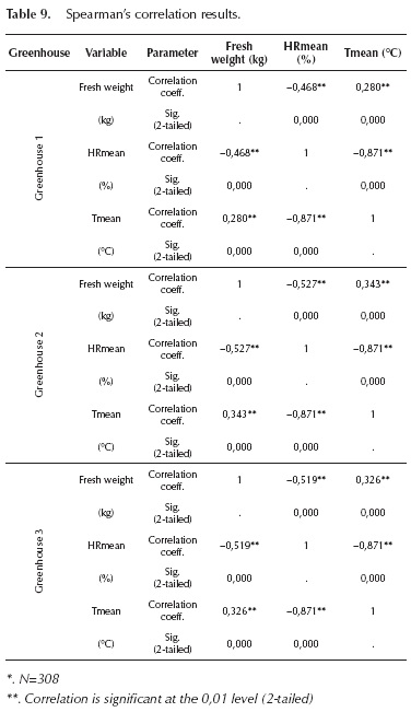
By analyzing the signs of the three correlation coefficients, it is shown that in all cases a significant negative correlation between the relative humidity and the fresh weight of the crop occurs. Similarly, regarding the temperature, there was a significant negative correlation between the relative humidity and the fresh weight. This is consistent with the production results obtained in the 3 greenhouses, where the 3^rd greenhouse, which was the warmest, had the highest production levels and, in turn, the 1^st greenhouse, which was the coldest, had the lowest yields. It is worth noting that the strongest coefficient was the one from the reverse correlation between temperature and relative humidity, which is explained by the strong inverse relationship of the variables discussed above.

Heteroscedasticity analysis

After statistically checking the influence of the relative humidity and temperature in the production of each crop for each greenhouse, an analysis of the behavior of the variation in both climate variables among the 3 greenhouses was done, regardless of the response variable. This is done to be able to conclude statistically the presence of different microclimates among the three greenhouses evaluated.

In order to do that, an analysis of variance of two variables - evaluating the behavior of their minimum, maximum and average in both cases - was carried out, so that the analysis goes from 2 to 6 variables. Table 10 shows the descriptive statistics obtained.

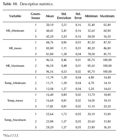
In all cases, the standard deviation was similar among the analyzed variables, so you can compare the average values to each other directly, as this implies that the data have a similar variation with respect to its mean. In the three greenhouses, the temperature shows a similar behavior as to the order of values. In all three cases the coldest greenhouse was the 1^st, and the warmest greenhouse was the 3^rd. Comparing the mean of minimum temperatures, the difference between these two greenhouses was 0,37 °C; while the difference with the 2^nd greenhouse was 0,29 °C. Regarding the mean of the average temperatures, the difference between the 1st and the 3rd was 1,42 °C and 1,13 °C between the 2^nd and the 3^rd. Finally, the difference between the mean maximum temperatures was 3,56 °C between the 1st and the 3^rd; and 3,21 °C between the 2^nd and the 3^rd.

As for the relative humidity variables, in the minimum and average variables it showed an opposite behavior with respect to temperature, which was expected by the negative correlation that occurs between these two variables. The greenhouse with the lowest average and minimum relative humidity was the 3^rd greenhouse, and the one with the highest values was the 1st greenhouse, with differences of 6,9 percentage points in the mean of the minimum variable and 2,96 percentage points in the mean of the averages. The differences between the 3^rd greenhouse and the 2^nd one were 5,23 and 2,10 percentage points, respectively. With respect to the maximum variables, no significant differences were found because there is a clear tendency to find values very close to 100 % almost every day in the morning, both outside and inside the greenhouses.

To confirm statistically that differences between the descriptions are meaningful, an ANOVA variance analysis was done (Table 11), starting from the null hypothesis that the mean of each of the variables is the same for the three greenhouses.

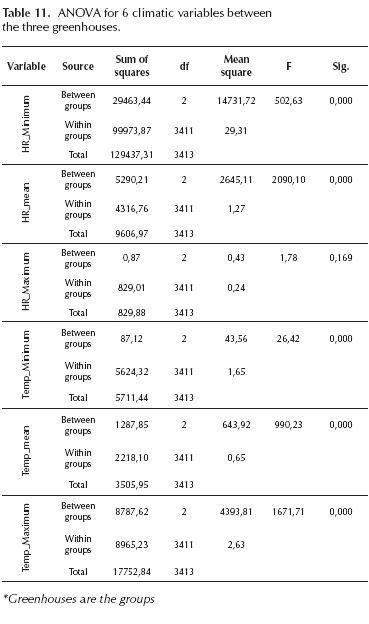
The comparison of statistical F resulted in the null hypothesis to be rejected in all cases (Sig. = 0,000), except in HRmean. This means that for a confidence level of 95 °%, it can be said that there were significant differences in the other 5 variables (T_Min, T_Med, T_Max, Hr_Min and HR_Max).

Conclusions

For a confidence level of 95 %, it is concluded that by reducing the minimum height channel from 3 m to 2 m, there is a difference in the microclimate of the greenhouse in the study. This produced an increase of 4,78 °% in the production of mint, which resulted in an increase of income.

The microclimate generated in each greenhouse is described by the differences in the 5 variables with which the heteroscedasticity analysis (T_Mean, T_Min, T_Max, HR_Min and HR_Mean) was made. It is concluded that for a confidence level of 95 °%, the reduction of 1m in the minimum height of channel resulted in an increase in minimum temperature of 0,37 °C, an average temperature increase of 1,42 °C and a maximum temperature rise of 3,56 °C.

In the case of relative humidity, the reduction of 1 m at a minimum height resulted in a decrease in the minimum relative humidity of 6,9 percentage points and 2,96 percentage points in the average relative humidity. The inverse relationship happened between relative humidity and temperature due to the high negative correlation statistically shown between these two variables by the three statistical correlation methods and the Durbin Watson statistical.

For a confidence level of 95 °%, it was shown that there is certainly a significant linear relationship between the joint interaction of relative humidity and temperature and the production of mint crops in each of the greenhouses.

References

Acuña, C., J. F. (2001). Nociones básicas sobre invernaderos,1^a edición. Bogotá: Publicaciones Facultad de Ingeniería Universidad Nacional de Colombia.         [ Links ]

Bareño, P. (2006). Hierbas Aromáticas Culinarias para Exportación en Fresco, Manejo Agronómico, Producción y Costos. Bogotá: Universidad Nacional de Colombia. PMid:16980408.         [ Links ]

Clavijo, J. P. (2006). Últimas Tendencias en Hierbas Aromáticas Culinarias para Exportación en Fresco. Bogotá: Produmedios.         [ Links ]

Dahlgren, J. P., Von Zeipel, H., & Ehrlen, J. (2007). Variation in vegetative and flowering phenology in a forest herb caused by environmental heterogeneity. American Journal of Botany. 94, 1570-1576. DOI: 10.3732/ajb.94.9.1570.         [ Links ]

Gonzalez-Real, M. M. (2009). La Gestión del Clima Bajo In­vernadero y Modelos de Simulación para su Manejo. Cur­so. Almería, España. PMid:19203958.         [ Links ]

Kleinbaum, D.G., Kupper, L.L., & Muller, K. (1988). Applied Regression Analysis and Other Multivariate Methods. Kent: PWS-KENT Publishing Company. PMid:3395499.         [ Links ]

Lambers, H., Pons, T. L., & Chapin, S. (2008). Plant physiologi­cal ecology 2nd edition. New York: Springer Verlag. DOI: 10.1007/978-0-387-78341-3.         [ Links ]

Pardo, M., & Ruiz, D. (2005). Análisis de datos con SPSS 12 Base. Madrid: McGraw-Hill.         [ Links ]

Portilla, A. (2007). Entorno de la Cadena productiva de las Plantas Aromáticas, Medicinales y Condimentarias en Colom­bia. Bogota: Universidad Nacional. PMCid:PMC2684501.         [ Links ]

Roy, J.C., Boulard, T., Kittas C., & Wang S. (2002). Convective and Ventilation Transfers in Greenhouses, Part 1: the Green­house considered as a Perfectly Stirred Tank. Biosystems Engineering. 83, 12-14. DOI:10.1006/bioe.2002.0107.         [ Links ]

Quintero-Arias, G., & Acuña, & C., J F. (April 2014). Incidencia de las películas plásticas en la variación de factores abióticos para la producción de lechuga en ambientes protegidos. En: VI Edición la conferencia Científica Inter­nacional sobre Desarrollo Agropecuario y Sostenibilidad "AGROCENTRO' 2014". Conferencia dirigida por Univer­sidad Central "Marta Abreu", Las Villas, Cuba.         [ Links ]

Sadras, V. O., Echarte, L., & Andrade, F. H. (2000). Profiles of Leaf Senescence During Reproductive Growth of Sun­flower and Maize. Annals of Botany. 85, 187-195. DOI: 10.1006/anbo.1999.101.         [ Links ]

Salisbury, F. B., & Ross, C. W. (2000). Fisiología de las plantas (Vol. Desarrollo de las plantas y fisiología ambiental). México D.F.: Grupo editorial Iberoamericana.         [ Links ]

Sherry, R.A., Zhou, X.H., & Gu, S.L. et al. (2007). Divergence of reproductive phenology under climate warming. Proce­edings of the National Academy of Sciences of the United States of America. 104,198-202. DOI: 10.1073/pnas.0605642104.         [ Links ]