DOI: http://dx.doi.org/10.15446/ing.investig.v36n2.55746

Segmentation of color images by chromaticity features using self-organizing maps

Segmentación de imágenes de color por características cromáticas empleando mapas auto-organizados

F. García-Lamont¹, A. Cuevas² and Y. Niño³

¹ Computer Science Ph.D, CINVESTAV-IPN. Affiliation: Universidad Autónoma del Estado de México, México. E-mail: fgarcial@uaemex.mx.
² Computer Science Ph.D, CIC-IPN. Affiliation: Universidad Autónoma del Estado de México, México. E-mail: almadeliacuevas@gmail.com.
³ Masters in Computer Science, COLPOS Montecillos. Affiliation: Universidad Autónoma del Estado de México, México. E-mail: yeninom@uaemex.mx.

How to cite: García-Lamont, F., Cuevas, A., & Niño, Y. (2016). Segmentation of color images by chromaticity features using self-organizing maps. Ingenie­ría e Investigación, 36(2), 78-89. DOI: 10.15446/ing.investig.v36n2.55746.

ABSTRACT

Usually, the segmentation of color images is performed using cluster-based methods and the RGB space to represent the colors. The drawback with these methods is the a priori knowledge of the number of groups, or colors, in the image; besides, the RGB space is sensitive to the intensity of the colors. Humans can identify different sections within a scene by the chromaticity of its colors of, as this is the feature humans employ to tell them apart. In this paper, we propose to emulate the human perception of color by training a self-organizing map (SOM) with samples of chromaticity of different colors. The image to process is mapped to the HSV space because in this space the chromaticity is decoupled from the intensity, while in the RGB space this is not possible. Our proposal does not require knowing a priori the number of colors within a scene, and non-uniform illumination does not significantly affect the image segmentation. We present experimental results using some images from the Berkeley segmentation database by employing SOMs with different sizes, which are segmented successfully using only chromaticity features.

Keywords: Segmentation of color images, color spaces, competitive neural networks.

RESUMEN

Usualmente, la segmentación de imágenes de color se realiza empleando métodos de agrupamiento y el espacio RGB para representar los colores. El problema con los métodos de agrupamiento es que se requiere conocer previamente la cantidad de grupos, o colores, en la imagen; además de que el espacio RGB es sensible a la intensidad de colores. Los humanos podemos identificar diferentes secciones de una escena solo por la cromaticidad de los colores, ya que representa la característica que nos permite diferenciarlos entre sí. En este artículo se propone emular la percepción humana del color al entrenar un mapa auto-organizado (MAO) con muestras de cromaticidad de diferentes colores. La imagen a procesar es transformada al espacio HSV porque en tal espacio la cromaticidad es separada de la intensidad, mientras que en el espacio RGB no es posible. Nuestra propuesta no requiere conocer previamente la cantidad de colores que hay en una escena, y la iluminación no uniforme no afecta significativamente la segmentación de la imagen. Presentamos resultados experimentales utilizando algunas imágenes de la base de segmentación de Berkeley empleando MAOs de diferentes tamaños, las cuales son segmentadas exitosamente empleando únicamente características de cromaticidad.

Palabras clave: Segmentación de imágenes de color, espacios de color, redes neuronales competitivas.

Received: March 28th 2016 Accepted: July 29th 2016

Introduction

Image segmentation is an issue widely studied to extract and recognize objects in a scene, depending on specific features such as texture, color or shape. The segmentation of color images has been applied in different areas such as food analysis (Gökmen and Sügüt, 2007; Lopez, Cobos and Aguilera, 2011), geology (Lepistö, Kuntuu and Visa, 2005), medicine (Ghoneim, 2011; Harrabi and Braiek, 2012).

Previous works have employed several techniques (Aghbarii and Haj, 2006; Carel et al., 2013; Liu et al., 2012; Mignotte, 2010; Mignotte, 2014; Rashedi and Nezamabadi-pour, 2013); but, most of them employ cluster-based methods, particularly Fuzzy C-Means (FCM) (Guo and Sengur, 2013; Huang et al., 2011; Kim, 2014; Mujica-Vargas, Gallegos-Funes and Rosales-Silva, 2013; Nadernejad and Sharifzadeh, 2013; Wang and Dong, 2012). By employing cluster-based methods, groups of colors with similar characteristics are created. The drawback of these methods is that they require a priori knowledge of the number of groups of data to be clustered. Thus, the number of groups is defined depending on the nature of the scene in order not to lose scenic color features. Other works employ neural networks (NN), which are trained with the colors of the given image, but they must be trained every time a new image is given (Ong et al., 2002; Zhang, Fritts and Goldman, 2008).

Humans identify the colors mainly by the chromaticity, then by the intensity. For instance, if the reader is asked to tell the names of the square colors (a) and (b) in Figure 1, the reader will answer "green"; note that the square (a) is brighter than square (b), but the chromaticity is the same. However, we claim that both squares have the same color but with different intensities.

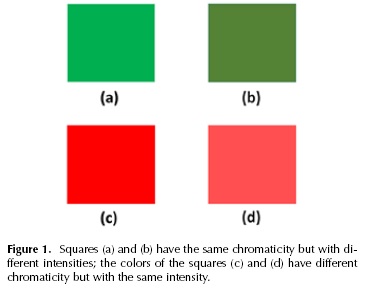
On the other hand, if the readers are asked to tell the names of the square colors (c) and (d) of Figure 1, they would answer "red and pink", respectively. In this example the intensity is the same in both squares. The chromaticity difference between both squares is small, but it is easy to appreciate the colors of squares (c) and (d) are not the same, despite both squares having the same intensity.

Humans, by observing their environment, can recognize objects and/or regions within a scene, to some extent, by the chromatic features. It is important to mention that humans are capable of recognizing colors. It is not necessary to identify them every time a new image is given, employing the knowledge acquired previously.

In order to emulate this human capability, we propose to train a self-organizing map (SOM), a kind of competitive NN, with chromaticity samples. After the SOM is trained, it is employed to segment images by their chromatic features. It is important to remark that the number of neurons of the SOM defines the number of colors the NN can recognize, which does not mean the image is segmented strictly with the same number of neurons. Each neuron activates when a given color is equal or similar to the one they learnt to recognize. There are neurons that do not activate because the colors they can recognize are not present in the image. Thus, the number of neurons reflects the maximum number of sections an image may be segmented into; while if FCM are employed, the images are segmented exactly with the number of clusters defined a priori. Hence, the contribution of this paper is a proposal for color image segmentation by using chromatic features, emulating the human color perception. A SOM is trained with chromaticity samples of different colors; the chromaticity of each pixel's color is extracted and then fed to the SOM, and the pixel is assigned the hue of the winning neuron. With this approach, any image is segmented without training again the NN and without knowing a priori the number of colors within the scene.

Proposed approach

Because of the fuzzy nature of colors, it is not possible to define limits between each color. However, it is possible to group the colors according to the hue features; for instance, pink hues can be grouped with red hues or cyan hues with green hues.

Our proposal consists on segmenting the images using the chromatic features of the images' colors. A SOM is trained with chromaticity samples of different colors; the chromatic feature of each pixel of the given image is extracted and then it is fed to the previously trained SOM. Then, the pixel is assigned the hue of the winning neuron.

RGB and HSV color spaces

The RGB space is a Cartesian coordinate system; the colors are defined as vectors extending from the origin (Gonzalez and Woods, 2002), see Figure 2.

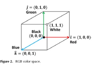
The color of a pixel p is a linear combination of the basis vectors Red, Green and Blue (RGB), written as:

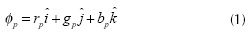
where the scalars r, g and b are the RGB components, respectively. The orientation and magnitude of the vector define the chromaticity and intensity of the color, respectively (Gonzalez and Woods, 2002).

The color representation in the RGB space is not the way humans perceive colors (Ito et al., 2006). For color classification, the cluster-based methods are not adequate for this space, because the difference between two colors cannot be measured using the Euclidean distance (Ong et al., 2002) if two vectors with the same orientation but with different magnitudes represent different colors. For instance, in Figure 1 the color vectors of the squares (a) and (b) have the same orientation, but they have different magnitudes, thus, they represent different colors.

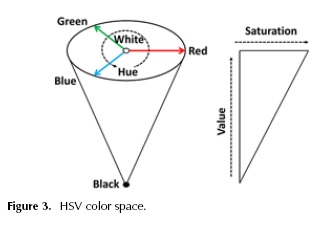
Previous works (Gonzalez and Woods, 2002; Ito et al., 2006; Rotaru, Graf and Zhang, 2008) claim the representation of color using HSV mimics the human perception of color because the chromaticity is decoupled from the intensity (Ito et al., 2006); hence, we employ this space. The HSV space is cone-shaped (see Figure 3). The color of a pixel p in this space has the elements hue (h), saturation (s) and value (v). That is:

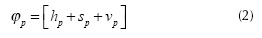
where hue is the chromaticity, the saturation is the distance to the glow axis of black-white, and the value is the intensity. Black is located at the tip of the cone and white at the center of the cone's base. The ranges of the hue, saturation and intensity are [0,2 π], [0,1] and [0,255], respectively.

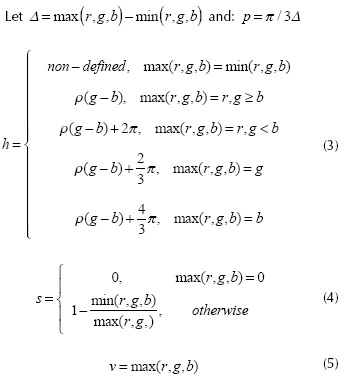
Usually, the colors of the acquired images are represented in the RGB space; thus, so as to process the images under our ap-proach, firstly the colors of the image are mapped to the HSV space. Mapping a RGB vector Φ = [r,g,b] to the HSV space is performed by using the following equations.

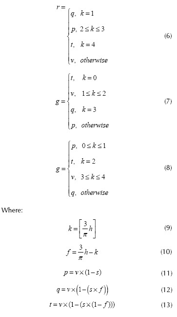
Mapping a HSV color vector Φ =[h,sv] to the RGB space involves the following operations (Gonzalez and Woods, 2002):

Proposed neural network architecture

The size of the NN depends on the number of elements to recognize. It is not possible to recognize the colors of the whole spectrum because of their fuzzy nature. But colors with similar hues can be grouped to divide the spectrum into a finite number of colors. If the SOM with a large number of neurons is employed, the segmentation may be poor; that is, if the chromaticity difference between two colors is small, given the large number of neurons assigned to different groups. On the other hand, if the NN has a few neurons, two colors can be assigned to the same group despite the chromaticity difference between two colors being large. Thus, in the experimental section, we process images using SOMs with different sizes.

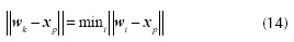
The SOM is a kind of competitive NN: it is based on finding the winning neuron before external stimuli. In other words, the output neurons with weights w_k compete between them so as to find the best match with the external pattern. We employ the Euclidean distance to measure the match between neuron w_k and the external pattern x_p. The neuron k whose weight vector w, is the closest to x is declared the winner, that is:

The winner and all the neurons within a neighborhood are updated by the Kohonen (1990) learning rule:

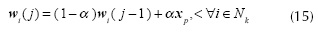
where 0 < α< 1 is the learning rate, j is the number of iteration and is the set of indexes of the neighbor neurons of the winning neuron k at a distance less than or equal to 1.

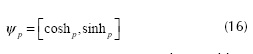
The chromaticity is represented as a vector because of the case when the hue is almost 0 or 2π. Consider squares (c) and (d) in Figure 1: the hue values are π/100 and 9π/100, respectively. Numerically, both values are very different, but the chromaticity is similar; if we classify the chromaticity of both squares only by their scalar hue values, for this case, the chromaticity will be recognized as if they were very different.

Hence, the scalar value is transformed into a 2-dimensional vector, where its magnitude and orientation are 1 and the hue, respectively. Let be the color of a pixel p in the HSV space, the chromaticity is represented as:

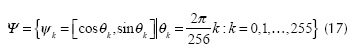
With this chromaticity representation, the problem mentioned before is overcome. As stated previously, the SOM is trained with chromaticity samples of different colors; the training set is built as follows:

The L*a*b* space is similar to the HSV space because in both spaces the chromaticity is decoupled from the intensity. We select the HSV space because the number of chromaticity samples, for the training set, is lower than if we use the L*a*b* space. That is, the chromaticity in the L*a*b* space is defined by the components a* and b*, where the range of both components is [-128,127] Thus, considering increments of 1 for the training set, there would be 255 x 255 = 65025 samples; with our approach the training set contains 255 samples. The number of chromaticity samples may be reduced if the L*a*b* space is employed, but it may lead the NN to recognize less colors.

The SOM cannot recognize white or black because they do not have a specific chromaticity; white can be defined as a low saturated color while black as a low-intensity color. Thus, before the pixel color is processed by the SOM, the color saturation and intensity must be analyzed to determine whether the color is white or black.

Hence, processing the pixel color involves the following steps: let , the color vector of pixel p represented in the RGB space,

1. The vector Φ_p is mapped to the HSV, where the vector is obtained.

2. If then v*_p and S*_p are set to zero, go to step 5.

3. If , then set v*_p to 191 and s*_p to zero, go to step 5.

4. If then:

1. Obtain vector Ψ_p and feed it to the SOM.
2. Obtain the weight vector of the winning neuron
3. The pixel p is labeled with the number of the win­ning neuron.
4. Compute the orientation of the weight vector of the winning neuron with Equation (18) and assign it to the hue component of the color vector.
5. Set s*_p to 1 and v*_p to 191.

5. Map the vector to the RGB space.

6. End.

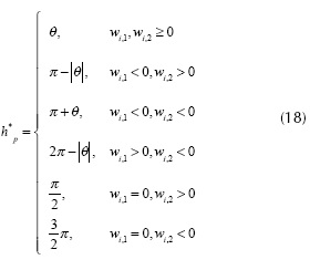
Where and δ_s and δ_v are the threshold values for saturation s v and intensity, respectively, and θ = tan^-1 (w_i,2,w_i,1).

Experiments and results

The number of colors the SOM can recognize depends on the number of neurons; hence, we perform tests with four SOMs with different sizes. The first, second, third and fourth SOM with 9, 16, 25 and 36 neurons are set in arrays of 3 x 3, 4 x 4, 5 x 5 and 6 x 6, respectively. The tests are performed using images of the Berkeley Segmentation Database (BSD), which is becoming the benchmark to test algorithms related to color image segmentation (Guo and Sengur, 2013; Harrabi and Braiek, 2012).

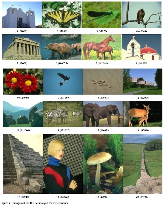
The BSD contains 300 color images and the size of the images is 481 x 321 or 321 x 481. Because of space constraints within the paper, we selected 20 images of the BSD to perform the experiments (see Figure 4). Figures 5, 6, 7 and 8 show the resulting images obtained after processing the images of Figure 4 using the SOMs with 3 x 3, 4 x 4, 5 x 5 and 6 x 6 neurons, respectively.

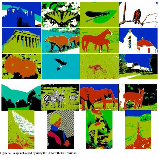
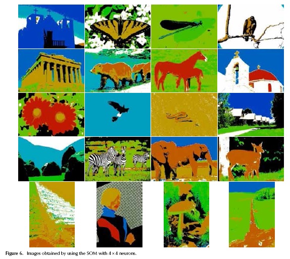
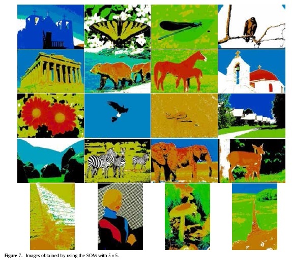
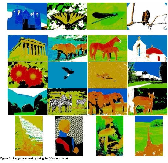
It is easy to appreciate that the resulting images can be segmented by using only the chromaticity features; but, also the segmentation of the images depends on the number of neurons of the SOM. That is, the larger the SOM is, the more colors are recognized; however, the segmentation is not always successful because some parts of the image are not segmented homogeneously despite the fact that they have the same color. In the following section the resulting images obtained are discussed and analyzed.

Discussion

The appearance of the images shown in Figures 5, 6, 7 and 8 is similar; there are some parts of the image segmented with different colors, but in others the segmentation difference is not easy to appreciate. In image 1 the church is segmented with the same blue hue using the SOMs with 3 x 3, 4 x 4, and 5 x 5. When employing the 6 x 6 SOM, the church is segmented with two different kinds of a blue hue. The area corresponding to the sky is not segmented with the same hue: with the SOMs 3 x 3 and 4 x 4 the sky is segmented with two kinds of a blue hue. The sky is segmented with four and three kinds of a blue hue, using the SOMs 5 x 5 and 6 x 6, respectively.

In the image obtained by processing image 17 with the SOM with 3 x 3, the hue of the segmented parts is homogeneous. With the other SOMs, the image is segmented into more parts with different hues that do not provide relevant data. For instance, in the images obtained with the SOMs 4 x 4 and 6 x 6, the stairs of the pyramid have two kinds of hue, while with the other SOMs the hue of the same part is more homogeneous.

By processing image 2, the difference can be appreciated in the hue of the butterfly's wings. Another difference is the green hue of the background, which is more homogeneous in the image obtained using the SOM 4 x 4.

Image 3 is essentially segmented into three parts: the insect, the leaf, and the background. In the image processed with the SOM with 3 x 3, all, or almost all, the background has the same green hue. When the size of the SOM increases, the hue of the background becomes less homogeneous. The larger the SOM, the more colors the SOM is capable of recognizing. Hence, more kinds of hue are assigned, while with a few neurons the opposite occurs.

The differences between the images obtained from image 4 can be appreciated in the small parts of the sky, which have two kinds of blue hue employing the SOMs with 4 x 4, 5 x 5 and 6 x 6; while with the SOM with 3 x 3 the sky is segmented with only one kind of blue. On the other hand, with all the SOMs the eagle and the leaf are segmented with the same hue; that is, the SOM with 3 x 3 is segmented with a red hue and with the other SOMs the same part is segmented with a brown hue. In image 5, the larger the SOM is, the more segments the image has. Using the SOM with 3 x 3, the building hue is homogeneous; while with the other SOMs the building is segmented with several hues. The sky is segmented with two kinds of hue in all the images obtained with the SOMs, although the segmentation of the sky with the SOM with 6 x 6 is different with respect to the images obtained with the other SOMs.

The images obtained by processing image 8 are very similar; the differences can be appreciated in the segmentation of the crosses and the top of the dome. With the SOMs with 3 x 3 and 4 x 4, the crosses have more than two kinds of hue; the dome is homogeneous with the same red hue. With the SOMs with 5 x 5 and 6 x 6 the opposite happens; the crosses have only one hue but the dome has two kinds of red hue, mainly on the top part. In all the images obtained, the sky is segmented homogeneously, each one with its own blue hue.

In image 9, the segmentation is better when the SOM has several neurons. Using the SOM with 3 x 3, the flower is not segmented clearly; with the other SOMs, the segmentation of the flower is clearer. The difference between these images is the background hue, although the segmentation is almost the same.

The appearance of segmented images obtained from image 10 is the same. The segmentation of the sky is uniform, each SOM with its own blue hue. Black and white, as mentioned before, are obtained thresholding the intensity and saturation of the colors, respectively, given that black and white do not have chromaticity.

The segmented images obtained by processing image 11 are almost the same. It is important to note that despite the color of the snake being very similar to the color of the sand, the SOMs are capable of distinguishing the hue difference, which could be difficult even for humans.

In image 18, the best segmentation is obtained using the SOM with 5 x 5 because details of the face can be appreciated. The case is similar using the SOMs with 4 x 4 and 6 x 6, but there is a stain on the face with the same hue of the hair. By employing the SOM with 3 x 3, the face is segmented homogeneously with the same hue. Note that in all the cases the skin hue of the face and the hand is the same.

It is easy to appreciate that the differences between the segmented images obtained by processing image 19 lie in the colors of the fungus, where the number of colors increases according to the size of the SOM employed. The brown hue of the background is different in each image obtained, while the hue of the green leaves does not change.

In the four images obtained by processing image 12, the sky is segmented homogeneously with the same blue hue. The area corresponding to the road is also segmented homogeneously. In image 13, the color of the mountains and the top part of the rocks are the same for the image obtained with the 3 x 3-SOM. The segmentation of the mountains is not totally homogenous using the SOMs with 3 x 3, 4 x 4 and 5 x 5 neurons. In all the images the grass, the rocks, and the sky are segmented with the same area and hue.

All the segmented images obtained from image 14 have the same area and color hues; except the image processed by the 4 x 4-SOM where several parts are segmented in a brown hue, and they should be segmented in a green hue. In image 15, the elephants are segmented homogeneously using the SOMs with 3 x 3 and 4 x 4; with the other SOMs, the elephants are segmented with two kinds of hue. In all the images the sky is segmented homogeneously with blue hue, except in the image segmented by the 5 x 5-SOM.

For the deer of image 16, the images obtained using the SOMs with 3 x 3 and 4 x 4 are segmented homogeneously, as well as the area corresponding to the grass. Using the SOMs with 5 x 5 and 6 x 6, the deer are segmented with two kinds of hue and the areas are different; the segmentation of the grass area is similar. Image 20 is essentially segmented into the wall, the sky, and the tree. The differences between the images obtained are found in the segmentation of the grass areas, while are segmented into different parts depending on the size of the SOM. The sky is segmented homogeneously, except when the 5 x 5-SOM is employed, where the sky is segmented with two kinds of a blue hue.

As we can appreciate in the images obtained, it is possible to segment the image by the chromaticity features. The number of colors to recognize in the image segmentation depends on the number of SOM neurons. For instance, in image 15 the number of segmented parts grows according to the size as the SOM increases; on the other hand, for images with few colors, the segmentation obtained is the same despite the size of the SOM, for instance, in image 10.

According to the quality of the images obtained, the best segmentation is obtained using the SOMs with 4 x 4 and 5 x 5. Moreover, the size of the SOM depends on the nature of the application or data extracted from the images. Due to the SOMs being trained with color chromaticity data, they cannot identify black or white because both colors do not have chromaticity. Black and white colors are recognized by thresholding the saturation and intensity values of the color, as mentioned previously.

Quantitative evaluation

The evaluation of color image segmentation has been subjective, but recently different metrics and defined ground truth images have been proposed in order to evaluate quantitatively the performance of segmentation algorithms of color images (Estrada and Jepson, 2009; Zhang, Fritts and Goldman, 2008). The BSD is becoming the standard benchmark to compute the performance of color image segmentation algorithms. As mentioned before, the BSD is a database of natural images; for each of these images the database provides between 4 and 9 human segmentations in the form of label maps which are employed as benchmark, ground truth images, to test quantitatively the performance of color image segmentation algorithms (Zhang, Fritts and Goldman, 2008).

Several metrics have been proposed, but absolute metrics have not been defined to evaluate the algorithms. We have observed in different papers (Wang and Dong, 2012; Mujica-Vargas, Gallegos-Funes and Rosales-Silva, 2013; Huang et al., 2011; Mignotte, 2010) the Probabilistic Rand Index (PRI) is becoming a standard metric; thus, we employ this metric to evaluate the segmentation of the resulting images.

The PRI compares the image obtained from the tested algorithm to a set of manually segmented images. Let {I,...,I_m} and S be the ground truth set and the segmentation provided by the tested algorithm. L^lk_i is the label of the x. in the kth manually segmented image, and L^S_i is the label of pixel x_i in the tested segmentation. The PRI index is computed with:

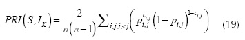
where n is the number of pixels, c_i,j is a Boolean function: 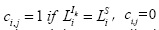otherwise; p_i,j is the expected value of the Bernoulli distribution for the pixel pair. The output range of the PRI metric is [0,1]; so, the closer to 1 the PRI value is, the more similar the segmented image obtained is with respect to the ground truth images.

Table 1 shows the segmentation values obtained from each segmented image with each of the SOMs employed. The highest values are obtained using the SOMs with 3 x 3 and 4 x 4 neurons. When the SOMs with several neurons are employed, the images obtained may have different segments that not always represent an important part of the image; for instance, image 10 obtained with the 6 x 6-SOM.

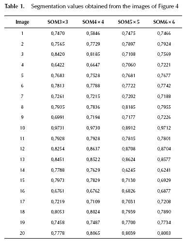
The values shown in Table 1 represent the probability that the segmented images and the human segmented images provided by the BSD are the same. The lowest value is obtained with image 1 using the 4 x 4-SOM; while the highest value is obtained with image 10 using the SOM with 3 x 3 neurons. The average values obtained with the 3 x 3, 4 x 4, 5 x 5 and 6 x 6-SOM are 0,7748, 0,7685, 0,7624 and 0,7683, respectively.

Conclusions

We have presented a proposal for color image segmentation by using chromaticity features. The self-organizing maps are trained with chromaticity samples to process the image colors. Related works on color image segmentation employ cluster-based methods, mainly fuzzy c-means. These methods require the user to define the number of groups or colors the image is divided into. Color image segmentation using self-organizing maps is not a novel idea; however, the difference with our proposal is that in the related works the neural networks are trained with the image colors to process. Hence, the neural networks must be trained for each given image. According to the resulting images, it is possible to segment color images using only chromaticity features.

With our proposal the neural network is trained only once with chromaticity samples, and it can be employed to segment any image without training it again. It does not require defining the number of image colors, as the cluster-based methods demand. The number of colors the neural network can recognize depends on the number of neurons, as shown in the resulting images of the Figures 5, 6, 7 and 8. The ideal size of the neural network, to process any image, cannot be defined; it depends on the nature of the application or the required data to extract from the images. But according to the quantitative evaluation and the appearance of the images obtained, the 4 x 4-SOM may be an adequate size for the neural network for this purpose.

The neural networks cannot identify black, white nor gray levels because the neural networks are trained to recognize just chromaticity; as future work, this issue can be addressed by using a fuzzy logic-based technique.

References

Aghbarii, Z. & Haj, R. (2006). Hill-manipulation: an effective algorithm for color image segmentation. Image and Vision Computing, 24(8), 498-903. DOI: 10.1016/j.imavis.2006.02.013.         [ Links ]

Carel, E., Courboulay, V., Burie, J. & Ogier, J. (2013). Dominant color segmentation of administrative document images by hierarchical clustering. ACM Symposium on Document Engineering, 115-118. DOI: 10.1145/2494266.2494303.         [ Links ]

Estrada, F. & Jepson, A. (2009). Benchmarking image segmentation algorithms. International Journal of Computer Vision, 85(2), 167-181. DOI: 10.1007/s1 1263-009-0251-z.         [ Links ]

Ghoneim, D. (2011). Optimizing automated characterization of liver fibrosis histological images by investigating color spaces at different resolutions. Theoretical Biology and Medical Modelling, 8(25), 2011.         [ Links ]

Gokmen, V. & Sugut, I. (2007). A non-contact computer vision based analysis of color in foods. International Journal of Food Engineering, 3(5), article 5. DOI: 10.2202/1556-3758.1 129.         [ Links ]

Gonzalez, R. & Woods, R. (2002). Digital image processing (Second ed.) Prentice Hall.         [ Links ]

Guo, Y. & Sengur, A. (2013). A novel color image segmentation approach based on neutrosophic set and modified fuzzy c-means. Circuits, Systems and Signal Processing, 32(4), 1699-1723. DOI: 10.1007/s00034-012-9531-x.         [ Links ]

Harrabi, R. & Braiek, E. (2012) Color image segmentation using multi-level thresholding approach and data fusion techniques: application to the breast cancer cells images. EURASIP Journal on Image and Video Processing, 11. DOI: 10.1186/1687-5281-2012-11.         [ Links ]

Huang, R., Sang, N., Luo, D. & Tang, Q. (2011). Image segmentation via coherent clustering in L*a*b* color space. Pattern Recognition Letters, 32(7), 891-902. DOI: /10.1016/j.patrec.2011.01.013.         [ Links ]

Ito, S., Yoshioka, M., Omatu, S., Kita, K. & Kugo, K. (2006). An image segmentation method using histograms and the human characteristics of HSI color space for a scene image. Artificial Life and Robotics, 10(1), 6-10. DOI: 10.1007/s10015-005-0352-x.         [ Links ]

Kim, J. (2014). Segmentation of lip region in color images by fuzzy clustering. International Journal of Control, Automation and Systems, 12(3), 652-661. DOI: 10.1007/s12555-013-0245-z.         [ Links ]

Kohonen, T. (1990). The self-organizing map. Proceedings of the IEEE, 78(9), 1464-1480. DOI: 10.1 109/5.58325.         [ Links ]

Lepisto, L., Kuntuu, I. & Visa, A. (2005). Rock image classification using color features in Gabor space. Journal of Electronic Imaging, 14(4), 1-3. DOI: 10.1117/1.2149872.         [ Links ]

Liu, Z., Song, Y., Chen, J., Xie, C. & Zhu, F. (2012). Color image segmentation using nonparametric mixture models with multivariate orthogonal polynomials. Neural Computing and Applications, 21(4), 801-811. DOI: 10.1007/s00521-011-0538-1.         [ Links ]

Lopez, J., Cobos, M. & Aguilera, E. (2011). Computer-based detection and classification of flaws in citrus fruits. Neural Computing and Applications, 20(7), 975-981. DOI: 10.1007/s00521-010-0396-2.         [ Links ]

Mignotte, M. (2010). Penalized maximum rank estimator for image segmentation. IEEE Transactions on Image Processing, 19(6), 1610-1624. DOI: 10.1109/TIP.2010.2044965.         [ Links ]

Mignotte, M. (2014). A non-stationary MRF model for image segmentation from a soft boundary map. Pattern Analysis and Applications, 17(1), 129-139. DOI: 10.1007/s10044-012-0272-z.         [ Links ]

Mújica-Vargas, D., Gallegos-Funes, F. & Rosales-Silva, A. (2013). A fuzzy clustering algorithm with spatial robust estimation constraint for noisy color image segmentation. Pattern Recognition Letters, 34(4), 400-413. DOI: 10.1016/j.patrec.2012.10.004.         [ Links ]

Nadernejad, E. & Sharifzadeh, S. (2013). A new method for image segmentation based on fuzzy c-means algorithm on axonal images formed by bilateral filtering. Signal, Image and Video Processing, 7(5), 855-863. DOI: 10.1007/s11760-011-0274-0.         [ Links ]

Ong, S., Yeo, N., Lee, K., Venkatesh, Y. & Cao, D. (2002). Segmentation of color images using a two-stage self-organizing network. Image and Vision Computing, 20(4), 279-289. DOI: 10.1016/S0262-8856(02)00021-5.         [ Links ]

Rashedi, E. & Nezamabadi-pour, H. (2013). A stochastic gravitational approach to feature based color. Engineering Applications of Artificial Intelligence, 26(4), 1322-1332. DOI: 10.1016/j.engappai.2012.10.002.         [ Links ]

Rotaru, C., Graf, T. & Zhang, J. (2008). Color image segmentation in HSI space for automotive applications. Journal of Real-Time Image Processing, 3(4), 311-322. DOI: 10.1007/s11554-008-0078-9.         [ Links ]

Wang, L. & Dong, M. (2012). Multi-level low-rank approximation-based spectral clustering for image segmentation. Pattern Recognition Letters, 33(16), 2206­2215. DOI: 10.1016/j.patrec.2012.07.024.         [ Links ]

Zhang, H., Fritts, J. & Goldman, S. (2008) Image segmentation evaluation: a survey of unsupervised methods. Computer Vision and Image Understanding, 110(2), 260-280. DOI: 10.1016/j.cviu.2007.08.003.         [ Links ]