


 English (pdf)
 Article in xml format
 Article references
 Send this article by e-mail
 Cited by SciELO
  Cited by Google
  Similars in
SciELO
Similars in
SciELO  Similars in Google
 Permalink
Introduction
The aim of this study is to improve a ground displacement velocity model along terrains with changing land cover, topographic and climatic conditions, including the slope direction of displacement as a key factor for determining optimal routes.
Normally, current displacement velocity models (Rees, 2004) calculate displacement time without considering upward/downward direction. These models take into account terrain slope from a digital elevation model, without sign, making the analysis incomplete. In this paper, we propose a velocity model including the upward/ downward direction of displacement. This model has been developed based on data from a topographic survey campaign using high-precision Global Positioning System (GPS) equipment, providing a great amount of coordinates and time for the calculation of velocity and slope. GPS data were processed by means of regression analysis for different terrain conditions. The model provides more reliable estimates of velocity displacement of personnel in the field and avoids possible problems in access and delays, among others, which allows establishing the variation of displacement velocity with respect to the slope.
Previous Work
Similarity between the path roads developed through time, due to the displacement of animals in pasturing grounds and the path roads generated by Geographic Information Systems (GIS) techniques was determined, indicating some relation of displacement with low energy trajectories (Ganskopp, Cruz, & Johnson, 2000). A procedure including surfaces of friction, sense of route of the slope and reclassification of land slopes with values from 1% to 91%, was implemented.
Some velocity models (Rees, 2004), based on investigations of times of long walks in mountainous lands, developed a quadratic model of velocity with respect to the slope, where it was established that the direction of the slope does not affect the displacement speed. This result does not agree with (Ganskopp, Cruz, & Johnson, 2000) where the effect of the direction of the slope was established by means of the great similarity between the calculated patterns and the observed ones in the field. The strong effect of the direction of the slope is evident; however, this single factor is evaluated by means of impedances in optimal routes determination but does not have a tangible physical meaning.
Classical procedures proposed in analysis of optimal routes, using georeferenced land coverage and elevation data in raster format, are based on the application of factors related to the slope and land use (Kang-Tsung, 2004). This procedure is incomplete because it does not take into account effects of the distance to the starting point, the topography, the geology, the crossroads, the rivers, and the proximity to populated centers. Additionally, it is necessary to evaluate the environmental impact caused by the intervention in the zone. These variables must be evaluated and classified through weighted factors to determine their influence.
A procedure for determining the velocity of displacement of tourists in a restricted network in Twelve Apostles National Park, in Victory, Australia, using the RBSim (Recreation Behavior Simulator) software, was proposed, obtaining reliable results for handling assigned employees and tourist resources (O'Connor, Zerger, & Itami, 2005). RBSim was developed by tracking some tourists through the implantation of a sensor in their ankle and monitoring them at six park locations. The analysis was made by means of known techniques of "quantitative ecology", like arrangement (ordering) that involved analysis of main components and factor analysis. The sampling did not allow obtaining diverse topologies differentiation, reaching the conclusion that the behavior of all the individuals was similar.
ArcGIS Software Manual describes the determination of the route of smaller cost (Least Cost Path) based on the reclassification of layers of land use and slope, assigning factors from 1 to 5 and from 1 to 10 for the first and second layer, respectively. Each layer is multiplied by subjective assigned weights values (i.e. 0,66 for slope, and 0,34 for land use). Finally, the cost map is obtained by adding these two layers in a grid format. This method does not consider the direction in which inclined terrains are passed through and the assignment of weights depend on the investigator's criteria.
There are recent works, related to field displacement velocity models, which consider the slope direction have to do with off-road dump trucks in construction and mining sites (Choi & Nieto, 2011), simulation of pedestrian movements in buildings to analyze people movements and route choice (Rivers, Jaynes, Kimball, & Morrow, 2014) , evaluation of different aged people walking in different slope terrain (Scaglioni-Solano & Aragón-Vargas, 2015) and, more recently, flow path modelling of people to support tsunami evacuation in disaster relief planning (Wood, Jones, Schmidtlein, Schelling, & Frazier, 2016). In spite of these researches, a pedestrian model related to field displacement in different terrains still has not been developed.
We propose a novel model that includes the sign of slope displacement (uphill and downhill) to calculate times for pedestrian displacement in order to implement it in Least Cost Path models where the impedance is the displacement time.
Materials and Methodology
Information about displacement velocity models was compiled from a GPS kinematic campaign along the Colombian territory, which consecutive pair of points was used to calculate displacement velocity and slope raw data. The information was processed by linear regression obtaining a model of slope versus velocity.
East and North coordinates were calculated at constant time intervals to obtain the velocity between each pair of stations. Other recorded information included the quality of coordinate determination error data RMS (Root Medium Square), topography surveyor ID and time was used as selection criteria. The velocity was calculated in m/s. The assigned value of RMS to each slope and velocity value corresponds to the average of RMS values of the determination of the two consecutive points used.
The data set was selected and grouped considering the quality and the minimal distance of displacement to consider real movement effectively. The quality was determined by the RMS values of the satellite points and the minimum range of displacement between the pair of consecutive points, considering the movement and discarding measurement errors.
The data was analyzed individually for each daily route of each surveyor, and then grouped by common geographic zones. Then, a regression was made for the complete dataset, analyzed in windows of distance and RMS values. Finally, the data was modelled by quadratic regression for each group of land use categories to obtain the RMS value that better adjust the data.
Slope and Velocity Data
Position of moving crews was determined by differential kinematics GPS, using ASTECH model STEP ONE instruments. This equipment has a precision of 1cm + 1ppm of the length of the base line. The length of the base line corresponds to the distance between the static equipment in the datum point (known as base) and the receiver that is in the point to be determined (known as rover).
Data acquisition was performed by the differential kinematic method, where the base and rover devices capture information simultaneously. The GPS Base is installed on a well-known station and the rover GPS collects East, North and Elevation data, along the route at a given time interval. This interval was settled to 10 seconds, within which the generation of a point of coordinates was guaranteed, controlling the displacement of the topographic crew. Coordinates with high RMS were eliminated. The precision of those GPS stations with high RMS is affected by the interference of the signal of the GPS due to the obstacles that impedes the arrival of the satellite signal to the antenna, for example vegetation, mountains, houses, buildings, etc.
Transient or auxiliary bases were tied between each other and occasionally tied to bench marks of the Geographic Institute Agustín Codazzi (or IGAC, from its Spanish initials), using the static differential method that consists on the generation of a line of control stations through the occupation of both points simultaneously, recording data during at least 45 minutes. All data was processed using the ASTECH SOLUTIONS software, which allows to obtain the coordinates of certain points, as well as the quality or error in the position known as the RMS.
Data was taken from a topographic survey that goes northwestward from the municipality of Aguazul (Casanare) to the municipality of Coveñas (Sucre) in the Colombian territory, along the Cusiana-Cupiagua Pipeline, which is approximately 800 km long. Due to the confidentiality of the information, data of coordinates are not included on this paper. Only slope and velocity estimations are enclosed from the consecutive positions of the points generated in the survey. The route passes along segments of the Departments of Casanare, Boyacá, Santander, Antioquia, Cordoba and Sucre. In Figure 1 main municipalities crossed by the topographical survey are displayed. The geographic regions from East to West are the Eastern foothills, the Cundinamarca-Boyacá high plain; the Western margin of the Eastern mountain range, the Middle Magdalena Valley, the Northern foothills of the Central range, the alluvial plains of the Cauca River and the savannahs of Cordoba. Each one of the crossed regions represents a wide spectrum of information associated to different terrain conditions to be evaluated.
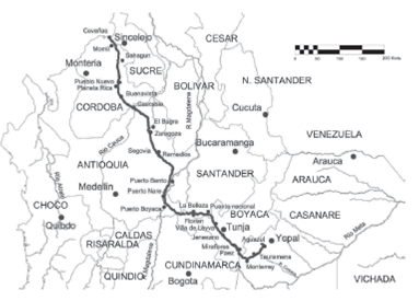
Due to the great variety of route conditions, the data was analyzed independently for each one of the 10 regions of homogenous conditions, trying to determine the incidence of climatic and geographic factors in the velocity model.
The topographic crew consisted of one surveyor and two local guides. The topographical survey was developed for two months with four topographic crews, working for three continuous weeks and resting one week. The crews were assigned based on their knowledge of the study areas. The velocities determined in this study can be considered as representative of average experienced topographic crew.
Data Processing
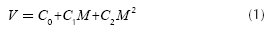
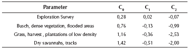
The applied regression of the data corresponds to a quadratic model (Rees, 2004), with the difference that in this case, the model is based on the velocity and not on the inverse of the velocity. Equation 1 represents the proposed model. In this model, the value of C1 is the parameter that indicates the effect of the direction used to cross the slope, whereas the value of C2 represents the effect of the slope magnitude.
Where:
V: |
Horizontal velocity. |
M: |
Slope of the terrain, (positive downslope, negative: upslope). |
C0: |
Independent parameter, velocity in flat terrain. |
C1: |
Effect of the direction to cross the slope. |
C2: |
Curvature - Effect of the slope magnitude. |
From Equation 1 |
the slope at which the maximum velocity can be obtained is estimated by: |
Determination of 1 constants was made by regression of clustered points which were closest to the regression curves in an iterative process. A single model for each homogeneous zone was generated to determine the effect of the regional conditions and slope in the velocity model. Each zone was evaluated and a quadratic regression for different number of clusters and for different values of RMS, establishing criteria that allowed considering only the information of displacement, rejecting other activities developed during the prospecting campaign.
During geophysical exploration surveys and topographic campaigns, various types of displacements occur that do not necessarily correspond to movement from a place to another place at normal speed. The following anomalous displacements could be identified:
Displacement error due to the precision of GPS instruments: This error is detected at a fixed station where the positioning solutions vary with respect to a fixed point (PDOP) due to the quality of the signal. This difference generates a "false displacement" and a false slope that do not correspond to the movement of the equipment. Apparent displacements can vary from few centimeters to some meters. To eliminate these estimates from the regression, values and minimum distance of displacement of the RMS are limited so that the point can be properly considered.
Displacements generated by the search of the ideal site to locate a GPS station: These displacements are slow and do not correspond to effective displacements at a normal speed. To eliminate these points from the regression, a minimum value of distance between points that depends on the conditions of the topographic survey is used. For effects of the regression, a minimum distance of 1m is selected to generate the velocity model corresponding to the search of the point.
In order to include the different types of land in the corresponding models of regression, it was required to group the data in homogenous zones, considering the geographic location, type of land, the slopes involved in the route and the varying RMS as well, to confirm the effect observed in the previous section.
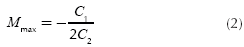
Figure 2 shows an example of the process of regression by means of grouping or clustering, made for two homogenous zones. The regressions were made for the different regions and values of the RMS and of the cluster, whose factors will be compared with the obtained velocity models.
The velocity model is representative of the speeds of each cluster or group. In Figure 3, the behavior of C1 is observed (the size of the point is proportional to the correlation coefficient for each curve).
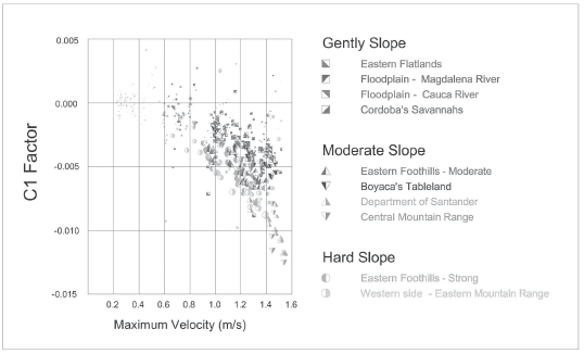
The different regions display a similar behavior grouping themselves around average values. The decrease of the displacement velocity in some flat regions is due to some exploration movements which could not be filtered. Nevertheless, the velocity solutions maintain coherence with the data collected for other regions.
It is important to write down that the variation of the maximum velocity towards negative slopes (descent) is evident in almost all clusters, with an exception for the low values of velocity that correspond to displacements while searching for the station site and not to the effective displacement of the survey along the pipeline.
It is evident that the movement of the maximum velocity is associated with the faster speeds of descending terrains, facilitating the displacement.
Figure 4 shows the variation of C2 indicating the curvature of the function. The negative value corresponds to concave curvatures, implying an evident reduction of the speed with the increase of the slope, without concerning the direction in which it is crossed.
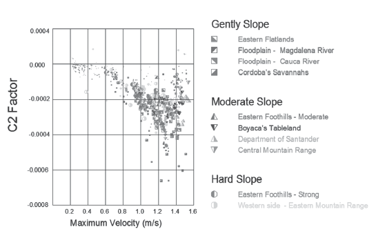
The behavior of model coefficients, for all the regions is similar and is concentrated around average values. In almost all the cases, this factor is negative and decreases as velocity increases, showing that the curvature grows, while walking along the terrain gets easier.
Due to the slight differences, it was decided to integrate all the coefficients in a single model, by means of the interpolation for each cluster. The four groups of curves were interpolated independently.
Results
According to the results of the quadratic regressions obtained in the previous section, velocity-versus-slope models were determined for each one of the types of terrains.
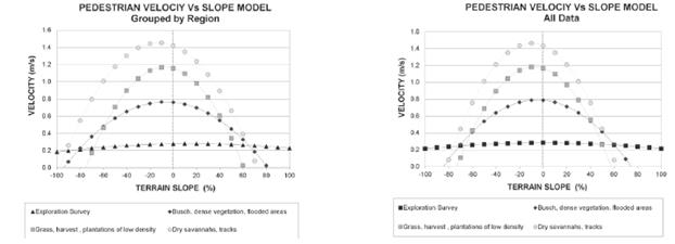
For this model, the characterization of the curves is obtained by regression. This characterization is merely descriptive and obeys to the interpretation of the results of the statistical groups by means of the Clustering. Figure 5 shows the results obtained from the average of C0, C1 and C2 factors for Clustering in three and four classes, with several values of RMS and minimum distance.
Final models are presented in Figure 5. The graph on top corresponds to the models interpolated in several types of terrains and conditions grouped by region while graph presented below corresponds to the model generated with all the data for all regions, in a single clustering process. Both models are practically equal.
The curves marked with circles correspond to the interpolation with four clusters. The curve with little squares corresponds to the interpolation with three clusters. In general, three zones can be defined: low, intermediate and high velocities.
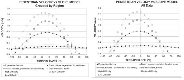
The low velocity zone from Figure 5 coincides remarkably. This zone of low velocity corresponds to very limited displacements searching for the station position. In this zone, the slope does not have any influence.
In the intermediate velocity zone, the maximum difference between regressions of the three and four clusters occurs. Figure 5 shows the central curve of the three clusters that correspond to the average curve of four clusters. The two intermediate velocity curves of the regression of four clusters allow the differentiation between displacement in difficult terrains such as scrubs, dense and low cultures flooded, and the little dense displacement in grass areas of smaller difficulty.
If the intermediate three cluster model is used, the terrain could only be considered as a non-differentiated intermediate difficulty zone.
Finally, in the zone of high speed, the regressions of three and four clusters agree, mainly because this is a zone of easy displacement that corresponds to footpaths and dry savannahs.
The maximum slopes of the model correspond to 90 % downslope and an 80 % upslope. This result shows the easiness to descend, compared to the difficulty to ascent. Additionally, at high slopes, the terrains must be crossed obliquely, trying to ascend (or to descend), reducing the value of the slope.
The effect of the slope associated with the direction of the route and the movement of the maximum towards the negative slopes (descent), becomes greater as the velocity of displacement increases.
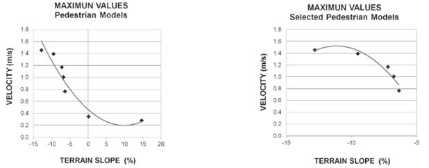
Figure 6 shows the increase of velocity with the slope corresponding to the maximum point of the function; it becomes more negative, so the final velocity model is reached after the down slope increases. Therefore, the effect of the sense of route measurement is increased as the down slope increases. It is possible to observe two points that do not seem to fulfill the hypothesis of the direction of the slope, but those points correspond to searching station sites displacements. If those points are eliminated, the maximum of this zone becomes more evident. Finally, the moving effect to the right of the curve is produced by the elimination of the two anomalous points.
Table 1 summarizes the model parameters for the velocity model and Figure 7 shows the definitive model using the final parameters.
Conclusions
The slope and type of land use of the terrain have strong influence in the modeling of velocity of displacement for moving land crews. Most importantly, the upward/ downward direction of the displacement is more critical, obtaining the maximum velocity models moving downslope.
In cases where the terrain does not present high difficulty, the effect of down slope/upslope is more significant. On the other hand, when the terrain is difficult to cross, the effect of downslope/upslope is diminished.
The variation of the velocity model with respect to the slope, has a quadratic behavior, especially where the coefficient that multiplies the slope is different than zero. Therefore, this coefficient cannot be ignored.
The model of velocity versus slope is very useful for planning fieldwork activities and for estimating the cost of fieldwork more efficiently. The impedance calculated for the fast routes imply less cost and more performance of technical crews and equipment.
The use of kinematic differential GPS data is very useful to calculate the displacement of personnel on the field by calculating models of velocity versus slope. Based on these models, it is possible to determine the efficiency of the people involved in the project to improve their performance in future works.
The modeling has been evaluated for potential field exploration programs. The results presented here can be expanded to seismic exploration programs, where more crews and equipment are mobilized.
The velocity versus slope model can also be applied in other disciplines in estimating evacuation routes, service network designs and rescue routes, among others. The model of velocity is also sensible to other climatic and anthropologic conditions not determined yet and should be considered in future works.
This model must be used to calculate optimal routes between points of exploration and evaluated in a practical field work.

