


 English (pdf)
 Article in xml format
 Article references
 Send this article by e-mail
 Cited by SciELO
  Cited by Google
  Similars in
SciELO
Similars in
SciELO  Similars in Google
 Permalink
Introduction
This paper presents the development of a seismic velocity model for the region of Bogotá, Colombia. Such models are a key ingredient for the physics-based simulation of ground motion in earthquake-prone regions, also called deterministic earthquake ground-motion simulations. The widespread damage caused by the 1994 Northridge earthquake provided the motivation for the development of the first three-dimensional (3D) velocity model ever in an effort to simulate earthquake ground motion in the greater Los Angeles Basin and gain a better understanding of its temporal and spatial distribution throughout the basin. Many velocity models have been developed since then. CVM-S, CVM-H, and WFCVM are some of the velocity models that have been widely used in the United States for simulating ground motions from past earthquakes as well as estimating basin effects from potential future earthquakes. CVM-S, the Community Velocity Model for Southern California - SCEC (Southern California Earthquake Center), incorporates contributions from multiple seismic and non-seismic data. The prototype, referred as version 0, is a geology-based 3D velocity model of the Los Angeles basin constructed from geologic information about crystalline basement, depth to sedimentary horizons, uplift of sediments, and surface geology in a velocity-depth-age function (Magistrale et al, 1996, 2000). The deeper sediment velocities are obtained from empirical relationships that consider age of the formation and depth of burial. The coefficients of these relationships are calibrated to sonic logs taken from boreholes in the region. Shallow sediment velocities are taken from geotechnical borehole measurements and hard rock velocities are based on tomographic studies. CVM-S4.26 is an improved version of this model that includes full 3D tomographic data as well as an optional geotechnical layer (GTL) implementation. A second model, CVM-H (Community Velocity Model - Harvard), describes the seismic P- and 5-wave velocities and densities of the crust and upper mantle structure in southern California. The first version was released in 2003 by Süss and Shaw (2003), and contains a P-wave seismic velocity structure derived from sonic logs and oil exploration reflection data in the Los Angeles basin, Vs is calculated from Vp using the relation "Brocher's regression line" (Brocher, 2005a). Density values are computed from Vp using the Nafe-Drake scaling relationship (Brocher, 2005a). CVM-H contains a GTL that describes the velocity structure in the shallow subsurface, where low shear wave speeds can have a significant impact on strong ground motions. Improvements in newer versions include revisions to the basement surface that incorporate the localization and displacements of faults in the Santa Maria Basin. Finally, the Wasatch Front Community Velocity Model (WFCVM) was developed by Magistrale et al. (2006) and covers the Wasatch Front region of North-Eastern Utah. The codes and model structure are based upon Magistrale's prior work on CVM-S. For the near-surface, the WFCVM interpolates the seismic velocities based mainly on isolated direct measurements (borehole logs) from previous studies and a detailed description of the basic geotechnical units given by MacDonald & Ashland (2008). For the deeper geological units in the crust, Moho and upper mantle, the WFCVM uses the results from a collection of studies including local earthquake travel times and standard one-dimensional (1D) models for earthquake location (Restrepo et al., 2012). Other models available for the United States are the USGS San Francisco Bay Area (Brocher, 2005b, and Brocher et al., 2006) and the central U.S. seismic velocity model CUSVM (Ramírez-Guzmán et al., 2012). As for previous, the development of the USGS San Francisco Bay Area and CUSVM required the compilation of crustal research consisting of seismic, aeromagnetic, and gravity profiles; geologic mapping; geophysical and geological borehole logs; and inversions of the regional seismic properties.
In Europe, some relevant models are: the Grenoble Basin (Chaljub et al., 2010) and Euroseistes (Manakou et al., 2010). The former considered seismic reflection profiles along the Isère Valley, together with information collected from boreholes drilled near Grenoble to calibrate or confirm the distribution of the sediment thickness in the valley, provided by gravimetric surveys and background noise H/V measurements. The model has two principal components: A 3D geometry consisting of free-surface topography, and a sediment-basement interface with a sediment and bedrock velocity models exhibiting only an 1D depth dependence (Chaljub et al., 2010). The geometric and dynamic properties of the 3D model of the Mygdonia basin geological structure (Euroseistes), in Northern Greece, were obtained from microtremor array measurements, seismic refraction profiles, boreholes and geotechnical investigations (Manakou et al., 2010). In addition, other models available for Europe are: The velocity model for the UK, Ireland and surrounding seas (Kelly et al., 2007) and the Po Plain sedimentary basin, Italy (Molinari et al., 2015). Koketsu et al., (2009) proposed a methodology for modeling regional 3D velocity structures in Japan. The methodology, initially applied to the Tokyo metropolitan area, was subsequently applied to northeastern, central and southwestern Japan, producing the integrated velocity structure model (JIVSM). The procedure consists of 7 steps that integrate different kinds of datasets, such as: refraction/reflection experiments; gravity surveys; surface geology; borehole logging data; microtremor surveys; and earthquake ground motion records. Additional models for Japan are the Kanto basin (Yamanaka and Yamada, 2006) and the 3D crustal S-wave velocity structure using micro seismic data recorded by Hi-net tiltmeters, developed by Nishida et al., (2007).
The first velocity model ever created of a seismic region in Colombia is for the Aburrá Valley Region (AVR). It was developed using geological units as a basis for determining the shear wave velocity. Restrepo et al., (2016) used 17 geological units studied by Acevedo (2011) and an artificial geologic unit of generic homogeneous material that was included to fill volumes where there was a lack of information. These geological units were incorporated into a computer algorithm that uses Delaunay triangulation to create interpolation rules to identify the corresponding geological unit enclosed by two adjacent sections (Restrepo et al., 2016). According to the Colombian seismic hazard study (AIS, 2010), Bogotá falls within an intermediate level of seismic hazard. This makes it desirable to develop a velocity model of this region, which would make it possible to simulate 3D ground motion in this region incorporating basin and local site effects.
Region of interest
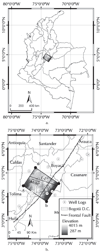
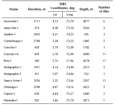
The region of interest is located in the Colombian Eastern Cordillera, in the region known as Cundiboyacense plateau, which includes Bogotá, some nearby towns, such as: Funza, Madrid and Cota, and is also bordered by the departments of Boyacá, Tolima and Meta. The city of Bogotá, capital district of Colombia, had a population larger than 7 million in 2011. Today it is the most productive city in Colombia, representing 26 % of the national gross domestic product, and approximately 50 % of the national tax revenue. The city is located in the Eastern range of Colombia, the widest branch of the Colombian Andes and has an urban area of 300 km2 and a population density of 3,53 people/m2, approximately. Bogotá is located in a zone of moderate to a high seismic hazard. Historically, it has been affected by the occurrence of strong earthquakes. Both, exposition and seismic vulnerability have been increasing at a considerable rate because of the massive migration and because approximately 75 % of the population has been growing in a disordered way (Yamin et al., 2013). Furthermore, the city was constructed on a lacustrine basin, with soft soils of considerable depth that could significantly amplify incoming seismic waves. Soil characteristics, seismic activity and the effects on the population that could produce the occurrence of strong seismic events are the motivations to improve knowledge about the soil properties in the region of Bogotá. A scenario containing a volume of the crustal structure of 131 x 102 x 70 km3 was selected. The coordinates in the World Geodetic System (WGS) and corresponding area are shown in Table 1 and Figure 1, respectively. The area is 13292 km2 and has a perimeter of 465 km. This polygon is bounded on the East by the Eastern plains and on the West by the Bogotá district area with an average topographic level of 2600 meters above sea level (m.a.s.l.). Furthermore, there is a contrast between a flat area (the plateau) and high mountains (Eastern Cordillera) that divide the area into two structural units: 1) a flat region shaped by a quaternary structure with a fluvial-lacustrine origin bordered by mountains of the Eastern Cordillera; and 2) a mountainous region characterized by mountains with steep slopes, deep canyons, and rounded shaped mountains composed of strong sedimentary rocks and soft clays shaped between the upper Cretaceous and upper Tertiary with heights that vary between the 2600 to the 3600 m.a.s.l. (Pérez, 2010).
Source: Authors
Figure 1 Location of the region of study. (a) Light-grey rectangle represents the 130 x 102 km2, targeted domain location in Colombia; (b) visualization of the digital elevation model and well logs location. The urban and rural areas of Bogotá are represented by a polygon filled with dots and the dotted line represents the frontal fault system.
Data and modeling approach
The methodology involved the following activities: (1) data collection, (2) data digitization, and (3) development of the model. These activities are described below.
Data collection
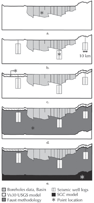
Geological and geotechnical studies were collected from public institutions such as the Bogotá aqueduct, Cundinamarca Regional Corporation (CAR, from its Spanish initials), National Hydrocarbons Agency (ANH), Colombian Geological Survey (SGC), and hydrogeological and geophysical private companies such as Hidrogeocol and GMAS. One of the most important types of documents gathered corresponds to the slowness vs. depth profiles obtained from sonic logging. Geological cross sections and a Digital Elevation Model (DEM) were also collected. Seismic well logs were obtained from oil companies studies available in the database of GMAS, a Colombian geoscience consulting company, and the ANH. These files are the basis for relating seismic properties to the reservoir, and comprise multiple petro-physical properties. However, only two types of data were used from these files: (1) compressional-wave velocities Vp calculated from the slowness logs, and (2) densities p which were obtained from the density logs existing in some of the wells. In total, 64 logs have been collected from 15 wells spread around the area of interest. In addition, a total of 12 geological cross sections were found in the data base of Hidrogeocol, a Colombian hydrogeology company. These geological sections were used to develop the 3D geological model with the software ArcGis 10.3 and its complement ArcHydro. In this study, four of the sections were extended to cover, end-to-end, the zones within the domain (see Figure 3). Information regarding topographic levels was downloaded from the free-access database ASTER GDEM, an easy-to-use, highly accurate DEM covering all the land on earth with a grid resolution up to 30 meters. Information collected, and wells utilized in the study are listed in Tables 2 and 3 , respectively.
Source: Authors
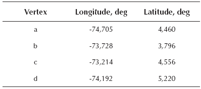
Figure 2 Scheme of the selection algorithm. (a) the grey irregular shape represents the basin where boreholes measurements are used to characterize the material properties; (b) grey rectangles represent the well logs coverage and are used to define material properties at points outside the basin and inside the shaded rectangle; (c) material properties at points above 30 m depth, outside the basin, and not covered by wells logs are characterized with the Vs30 USGS model; (d) wave velocities and density at points above 4 km depth and not covered with the datasets previously mentioned are characterized using the Faust methodology and, (e) the SGC 1D velocity model is used to characterized points at depths greater than 4 km.
Data digitization process
Several types of digitization process were selected according to the type of data. Since most of the relevant material was found as images, PDF files, and printed documents, the use of some image processing tools was necessary to obtain the necessary information. Data documented in well logs (densities and slowness) were extracted using a vectorization of TIFF images followed by an image processing using a program coded in Matlab. The results of this procedure were the values in depth of p and Vp for each well. Additionally, the geological cross sections were digitized from PDF files. Basically, these vertical profiles outline the spatial distribution of the geological units along a cut. To digitize theses profiles, an ArcGis tool was used to get coordinates x, y and z of the upper and lower boundaries of each geologic structure. Finally, the processing of the DEM was performed. The original version of the DEM was formed by 6 individual rasters that covered an area greater than the one of the polygon considered, and a significant number of unrealistic topographic peaks, that were corrected using ArcMap 10.3.
Development of the model
The methodology developed by Magistrale et al., (1996, 2000) was adapted to construct a geology-based 3D velocity model of the Bogotá region. The model required the construction of a crustal structure (or geological model) and a material properties model that depends on the crustal structure and data from: (1) geotechnical borehole measurements, (2) well logs, (3) USGS Estimates of site conditions from topographic slope, (4) a velocity-depth-age function, identified as Faust methodology to be described later in this article, and (5) the 1D wave velocity model from the Colombian geological survey (SGC, from its Spanish initials). The crustal structure is integrated into the velocity model by means of the Faust methodology, where the geological model is used as an input to obtain the seismic wave velocities and density. The velocity model is a computer algorithm that uses the coordinates of the point of interest to identify the dataset that best represents the material properties. The algorithm assigns the values of seismic wave velocities and density based on the horizontal coordinates and depth of the point of interest. As shown in Figure 2, shallow sediment velocities are characterized from: (i) geotechnical borehole measurements when the point is inside the Bogotá basin (Figure 2a), (ii) well logs if the point is located within a radius of 5 km from the well log horizontal coordinates (Figure 2b), or (iii) Vs30 values from the USGS estimates of site conditions from topographic slope when the point is at less than 30 meters deep and could not be characterized with any of the two previous datasets (Figure 2c). The deeper sediment velocities are obtained from: (i) an empirical relationship that considers age of the formation and depth of burial when the point is located at less than 4 km deep, and cannot be characterized with the datasets named above (Faust methodology, Figure 2d), and (ii) the SGC 1D wave velocity model for points located at depths larger than 4 km (Figure 2e). An interpolation or extrapolation is performed using a Delaunay triangulation of scattered sample points when the selected dataset corresponds to (2) or (3). Otherwise, the calculation of the material properties will vary depending on the dataset. A description of the geological model and the five datasets incorporated in the algorithm is shown below.
3D Geological model
The geological units define the groups of rocks characterized by common lithologic properties that differentiate them from adjacent units. In this study, some of the geological units are Guadalupe, Villeta, Sabana and Guaduas. Guadalupe (Ksg) is formed by four units: Arenisca dura (Kad), plaeners (Kp), labor tierna (Klt).
Ksg has a large variety of sedimentary rocks with thicknesses that vary between 550 meters in Facatativá and 750 meters in the Guadalupe hills. In addition, some rock properties may differ drastically between units. These variations sometimes complicate the visualization of other units, for example, Villeta (Kv), which in some localities has properties similar to Guadalupe (Lobo-Guerrero, 1992). Kv is a geologic structure composed by 8 units that are mainly formed by sequences of black shales of the Cretaceous. This formation is located under Guadalupe, delimiting the Eastern Cordillera between the units Naveta and Dura. Moreover, Sabana (Qs) is a surface quaternary formation with a maximum thickness of 320 meters, consisting mainly of sands and gravels with an important water storage capacity. Qs is divided into three particular units: Suelos de la Sabana (Qsb), Terraza Alta (Qta) y Terraza Alta (Qtb). Guaduas (Kpgg) is located in the middle of the eastern Cordillera; it was originated between the Tertiary and Cretaceous periods, and is known for its coal resources (Amaya et al., 2010). Kpgg consists of two distinguishable units: the lower unit formed by clays and brown shales of significant thickness, interspersed with sandy layers of variable thickness. The upper unit consists of alternating levels of continuous fine sandstones, gray and yellow clays and economically exploitable coal seams with thicknesses ranging from 0,60 to 4,0 m. A total of 124 geological units were found in 33 cross sections from previous studies (see Figure 3); they were matched and simplified to a total of 48 units. Additionally, four of the existing cross sections were extended to cover, end to end, certain areas of the domain (Montejo et al., 2016). A geospatial analysis was required to generate the 3D geological model. The geology model was obtained using Arc Hydro, a set of data models and tools that operate in the ArcGIS environment. Most of the Arc Hydro tools are geared to support water resources applications; however, additional tools have been developed for geoprocessing environments and can be used in ArcMap. These additional tools are part of the subsurface analyst feature, and are useful to manage and edit geolocated 2D sections to create 3D volumes, using the horizons method. XS2D geophysical plot features were used to create panels (similar to ArcGis 2D common polygons) that represent the geological units in each cross section, delineated by a bottom and an upper line; these upper and lower boundaries were transformed into rasters that represent the surface or horizons to interpolate between topographic levels with the inverse distance weighted method (IDW). The generated horizons were converted into GeoVolumes by filling empty spaces between the existing rasters. Representative results of the 3D geological model are shown in Figure 4.
Source: Authors
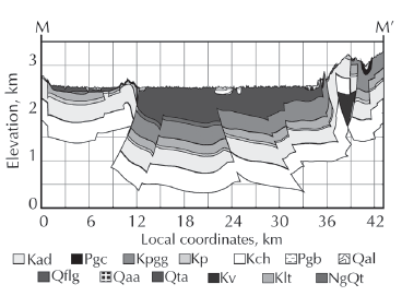
Figure 3 Geological cross section M-M'. Representation of the geological units on the vertical cut M-M'. The colors and patterns of the cross-section depict the geological units. Location of the cut on the domain is shown in Figure 1. Geological units and their correspondent nomenclature are listed below: arenisca dura (Kad); Cacho (Pgc); Guaduas (Kpgg); plaeners (Kp); Chipaque (Kch); Bogotá (Pgb); deposito aluvial (Qal); fluvio glacial (Qfl); depósitos de avanico aluvial (Qaa); depósitos terraza aluvial (Qta); Villeta (Kv); labor tierna (Klt) and Tilatá (NgQt).
Source: Authors
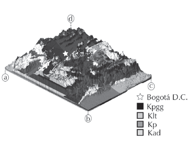
Figure 4 3D Geological Model. 3D representation of the crustal structure above sea level. Interpolated geological units are distinguished by colors, some representative geological units are identified (Guaduas - Kpgg, Labor tierna - Klt, Planers - Kp, and Arenisca dura - Kad). The star marker represents the location of Bogota in the model. Polygon's vertices are identified by letters a - d (corresponding coordinates are shown in Table 1).
Model datasets
Geotechnical borehole measurements: The results from the microzonation measurements were used to identify areas with similar geotechnical conditions within the Bogotá basin. In this case, the seismic zones of the microzonation were characterized by a single Vs vertical profile. These profiles were constructed using the 126 geotechnical boreholes from the microzonation. The mean value of all vertical profiles contained within the same seismic zone were used to determine a single vertical profile. Therefore, the properties of each single vertical profile will be assigned to any point within the corresponding seismic zone.
Well logs: Vertical profiles from well logging were associated to its corresponding coordinates and then the model properties are calculated at any point within the domain that is covered by these profiles. In this case, data coverage was defined as 5 km in any radial direction where the coordinates of the origin correspond to the well log coordinates. The maximum and minimum depth depend on the vertical profiles.
USGS Estimates of site conditions from topographic slope: This model correlates the average shear-velocity down to 30 m (Vs30) measurements against topographic slope to develop two sets of coefficients for deriving Vs30: one for active tectonic regions that possess dynamic topographic relief, and one for stable continental regions where changes in topography are more subdued (Allen & Wald, 2007). Both sets were downloaded and compared to the values of Vs30 calculated from the geotechnical borehole measurements using a kriging interpolation in ArcGIS. The misfit between the borehole measurements and the USGS estimates was calculated as the square root of the difference between the datasets. The selected set (active tectonic) corresponded to the one with the minimum misfit with respect to the microzonation measurements. In the study, the USGS estimates were used to characterize the shear-wave velocity of shallow sediments as a homogeneous layer of 30 m depth. The algorithm selects this dataset when there is no data from other sources (e.g. points located out of the basin or points not covered by well logs).
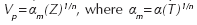
Faust methodology: According to Faust (1951), a relationship between compressional wave velocity, depth and age of the geological units can be established. This approach, previously implemented in the velocity model of Los Angeles basin, California, USA (Magistrale, 1996), was used to characterize points at depths between 30 m and 4 km when there was no other available data. Faust's methodology proposes the following relationship:
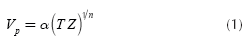
where Vp represents the compressional-wave velocity expressed in m/s, T is the geological age of each formation in millions of years, Z is the depth in meters and n and a are constant values. To arrive at this equation, Faust studied well logs from North America and determined a sediment age-depth-P-seismic-wave-velocity relation (Magistrale, 1996). In contrast to Los Angeles Model, there is no extensive information about the age and depth of sediments in the Bogotá region. The geological age and depth were obtained from exploration oil studies and geological cross-sections. Information about geological units, and its geologic period and age was found in 6 of the 13 well logs available (see Table 3). This data is listed in Table 4 (where Anaconda-1, Cormichoque-1, Corocito-1A, Pore-1, Coporo-1, and Chitasuga-1 are identified as wells 1, 2, 3, 4, 5 and 6). The methodology used to find a relationship between Vp, depth and age of the geological units, is summarized below:
Table 4 Geological data available in seismic wells. List of geological units and its corresponding geologic period, and age
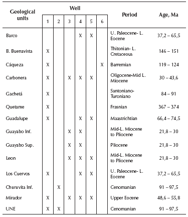
Source: Authors
The equation proposed by Faust (1951) (see Equation 1) was expressed as:
The value of αm was calculated using the oil exploration data. In this study, the value of αm was obtained from each pair of Vp and Z available in the wells logs. Initially, the value of n was assumed to be 6 (Faust Model). This power represents the tendency of the sediments to compact and harden as they are buried and they age (Magistrale,1996).
αm values are assumed to be log-normally distributed. This assumption was tested by constructing Q-Q probability plots of αm. This test was also performed for normal, Weibull and Rayleigh distributions. However, the log-normal distribution provided the best fit. Furthermore, αm must be a positive number and a random variable which is log-normally distributed will take only positive real values.
A total of 30 iterations were performed to determine the values of αand n. Each iteration consisted of 50000 Monte Carlo simulations with random values of αm (log-normally distributed) and T (a uniformly distributed variable that ranges between the ages of each geological units).
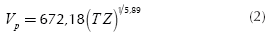
An exponential regression was evaluated in each Monte Carlo simulation to obtain the values of α and n. The mean values of α and n (corresponding to the 50 000 simulations) were used as an input for the next iteration. After 30 iterations, the values of α and n converged to 672,18 and 5,89, respectively. Consequently, the age-depth-P-seismic-wave-velocity relationship can be expressed as: Equation (2) can be used to determine the values of Vp in m/s at any point within the region. For any point with x, y and z coordinates, the geological age in millions of years, T, is determined from the geological model, and Z is the depth in meters.
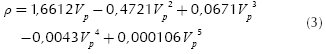
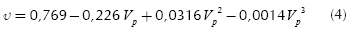
The density (ρ) and Poisson ratio (υ) were calculated as function of Vp using the corresponding relationships proposed by Brocher (2005a), shown here in see equations 3 and 4. The shear wave velocity (Vs) was then obtained using the standard relationship for the ratio Vp / Vs for elastic materials (see Equation 5).
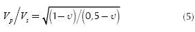
SGC 1D wave velocity model: This background model represents the variation of the wave velocities with the depth and was calculated using P-wave travel time from local seismicity (Ojeda & Havskov, 2001). This model is used by the Colombian Geological Survey (SGC) to locate earthquakes and has six layers over a half space (see Table 5). The average Vp / Vs for all layers is 1,78. The Vp values shown in Table 5 and the V / V ratio mentioned above are used to characterize the material properties in points at depths larger than 4 km.
Representative results
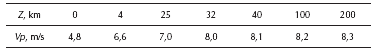
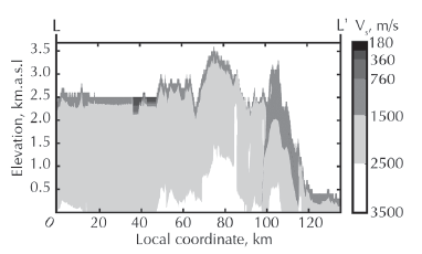
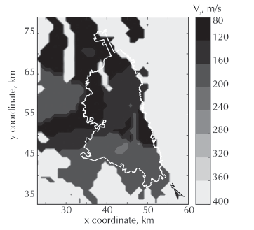
A location-based approach was adopted to calculate the seismic-wave velocities and soil densities at any point within the volume of interest. Some highlights of the program are: (1) the program does not interpolate between all the available data. The selection of the information used to determine the model properties at a given point depend on the point coordinates; (2) the highest resolution in the data can be encountered in the basin; and (3) to take advantage of the seismic zoning defined in the seismic microzonation of Bogotá, the program uses a single vertical profile per seismic zone instead of interpolating between vertical profiles within the same seismic zone. Representative results are shown in Figures 5 to 7. Figure 5 shows a contour map of Vs at the surface of the model (depth = 0 m), and Figure 6 shows the values of Vs along the cross-section L-L' (see Figure 1). As shown in Figure 5, the lowest values of Vs can be found in the Bogotá district and nearby towns. Similarly, the lowest values of Vs observed in Figure 6 coincide with the location of the Bogotá basin. This aspect is of interest because it confirms that the basin beneath Bogotá has soft material fills (Vs ≤ 400 km/s) that reach depths of up to 425 m. Finally, Figure 7 shows the variation of the shallow sediments shear-wave velocities at a local scale (urban area). The lowest values of V are concentrated in the north and center of the basin, where they vary between 80 and 150 m/s while higher values are observed in the south of the city. These shear-wave velocity variations in the basin are consistent with the Vs30 distribution developed by Pulido et al. (2016) using initial microtremor array measurements in the basin. We are aware that the well log information used to estimate parameters in equation 2, is only available outside the Bogotá basin and therefore might not precisely reflect the lithology of the basin. However, the velocity model for the basin is based on geotechnical boreholes from the microzonation and experts' interpretation of the geotechnical conditions of the city (C. Molano & A. Huguett, personal communication, 2016).
Source: Authors
Figure 5 S-wave velocity at the surface. The proposed S-wave structure reasonably detects the soft deposits of sediments in the basin (Vs ≤ 400 m/s).
Source: Authors
Figure 6 S-wave velocity distribution along the cross-section L-L'. The location of the cut L-L' is shown in Figures 1 and 5.
Concluding remarks
The velocity model of the Bogotá, Colombia region developed in this study has been implemented into a completely automated computer code. The user need only define the latitude, longitude, and depth of a point of interest within the region, and the model provides the corresponding values of the density, the P-wave velocity, and the shear-wave velocity at that point. By evaluating these properties at a set of points within a sub-region of interest, this model can be used for different applications, such as earthquake ground motion simulation in extended regions, microzonation, and site characterization. The data resolution at the basin will be improved by incorporating material properties obtained from microtremor observations (Pulido et al., 2016). Material attenuation has not been included in the model. It can be readily incorporated, for instance, as is done in the Community Velocity Models for southern California, by associating the amount of damping in the material at a point to the corresponding shear-wave velocity.

