Using Response Surface Methodology along with the Pareto Genetic Algorithm

The following subsections present some parts of the previous PGA (PGA1) and concepts related to RSM necessary for understanding the changes made to PGA1. More details of PGA1 may be found in ^{Canessa et al.(2014}).

Some details of the original Pareto GA (PGA1).

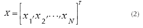
The previous PGA1 developed in ^{Canessa et al. (2014}) represents the combinations of k control factors that may take s different levels (values) of a robust design experiment using an integer codification. One chromosome will be composed of a combination of different levels for each factor, which corresponds to a particular treatment of the experiment. Let f _lj be the factor j of chromosome l, with j = 1,2, …,k and l = 1,2, …, N. Each f _lj can take the value of a given level of the factor j, that is 1,2,s. One chromosome (or solution) is expressed as a row vector (see Equation (1)). The matrix representing the total population of solutions X will be composed of N chromosomes (see Equation (2)).

Each of the chromosomes (solutions) ^_Xl will generate different responses ^_yr(r = 1,2,3,...,R) of a multi-response system when the control factors are set to the corresponding levels specified in the chromosome ^_xl. The PGA searches through the space of possible treatment combinations, finding the combinations that minimize the variance of the responses and adjust their means as close as possible to their corresponding target values. The problem that the PGA needs to solve can be expressed by Equation (3):

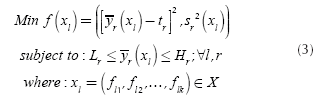
Expression (3) means that the PGA will try to find solutions x _l , which must adjust the mean of each response ^_yr to its corresponding target value ^_τr and simultaneously reduce the variance of each response. ^_Lr and ^_Hr are lower and upper limits within which, each response ^_yr is feasible and must be set by the engineer. Following the work presented in ^{Del Castillo, Montgomery & McCarville (1996)}, a penalty function is used to enforce such limits. Finally, in the case of single-response systems (R = 1), the PGA directly uses expression (3). On the other hand, for multi-response systems (R > 1), the PGA aggregates over all responses yr into φ1 using a desirability function proposed in ^{Ortiz et al. (2004}). The same is done with all the s2r to obtain φ2. Given that the desirability functions are defined so that the and s² _r the larger ^_φ1 and ^_φ2 (in the range [0,1]), the problem for multi-response systems is stated as a maximization of ^_φ1 and ^_φ2 as Equation (4) shows:

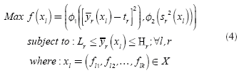
More details of these mechanisms may be found in ^{Canessa et al. (2014)} and are not repeated here for the sake of length and because an exhaustive explanation is unnecessary for understanding the work shown here.

From Equations (3) and (4), one can see that in the calculation of the value of those expressions PGA1 needs to know the responses corresponding to the experimental treatment, which each chromosome represents. However, some of those treatments might not have been part of the experiment that the engineer conducted to gather the data. Thus, PGA1 needs to estimate those responses. In PGA1, for estimating the mean of a response for a non-tried chromosome (treatment), PGA1 calculates the main effect of each of the treatment levels on the response and a grand mean using all the observations corresponding to the experiment that was carried out. Then, PGA1 adds to the grand mean the corresponding main effects of the levels indicated by the chromosome. For estimating the variance of the response for a non-tried chromosome (treatment), PGA1 uses a similar procedure. PGA1 first computes a global variance considering all the replications of all the treatments tried in the original experiment. Then PGA1 calculates the main effect of each control factor on the variance. Finally, PGA1 sums the main effects of the levels indicated in the chromosome to the global variance. Those procedures correspond to a linear estimation usually applied in the ^{Taguchi method (for a worked out numerical calculation, see example in Taguchi (1991}, p. 16). In the search process, PGA1 uses roulette or probabilistic selection, a uniform crossover with ^_pc = 0,3 and a bit by bit (factor by factor) mutation operator with ^_pm = 0,05. PGA1's stopping criterion is to iterate 15 times. Larger values of iterations were tried, but the performance of PGA1 did not improve (^{Canessa et al., 2014}). To implement PGA1, the Strength Pareto Evolutionary Algorithm 2 (SPEA2) (^{Laumans, 2008}) is used, with minor adjustments that the interested reader may find in Canessa et al. (2014).

RSM and its application to the estimation of missing values in the new Pareto GA (PGA2).

Using techniques that are part of Response Surface Methodology (RSM), ^{Vining & Myers (1990)} proposed the use of second order polynomials to adjust a surface that may represent the mean and variance of a system and employ that surface in optimization problems. Further analysis of that approach indicated that it provides many benefits (for a good discussion see ^{Nair, Taam & Ye, 2002}). ^{Vining & Myers (1990)} recommended the following expressions for estimating the mean and variance of the output of a system, based on the vector of k control factors (X):

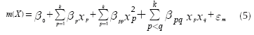
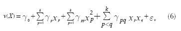
Expression (5) corresponds to the response surface that estimates the mean of the response and Equation (6) approximates its variance. Note that both expressions assume that each control factor x is a quantitative variable. However, it may be the case that some experiments might involve one or more qualitative variables. In such case, the researcher will need to represent those qualitative variables using indicator variables (Myers & Montgomery, 2002). Accordingly, Expressions (5) and (6) must be modified to accommodate the use of indicator variables as Equations (7) and (8) show:

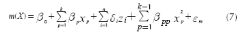
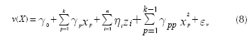
where there are k quantitative control variables, and z ₁ , z ₂ ,… ^_zn are n indicator variables, which represent the qualitative control variables. Also, the response surface assumes that there are no interactions between indicator and quantitative variables and among quantitative variables. If that occurs, the experimenter must add some terms to Equations (7) and (8), but commonly the researcher tries to avoid including those interactions (Myers & Montgomery, 2002), which agrees with ^{Taguchi's suggestions for conducting parameter design experiments (Taguchi, 1991}, cf. ^{Roy, 2001}).

To estimate the response surfaces characterized by Expressions (5) and (6) or (7) and (8), the Ordinary Least Squares (OLS) regression method is generally used (Myers & Montgomery, 2002). Thus, the modified PGA (PGA2) applies specific versions of Expressions (5) through (8) and implements an OLS routine to estimate the response surfaces corresponding to the mean and variance of each output. Then, PGA2 uses those surfaces to approximate the mean and variance of an output, if such values are not directly available from the data collected from the robust design experiment that was carried out. Since the response surface for the variance is only an estimation of the true and unknown surface, it could happen that a missing value of variance estimated by the surface might be inappropriate, i.e. negative. That may occur because PGA2 is estimating a value outside the range of the values of the control factors used in calculating the regression, i.e. it is extrapolating, or simply because the estimated surface is not totally representative of the behavior of the variance of the system. Therefore, the algorithm verifies whether the estimated variance is negative and, if that is the case, it estimates the variance again using the original approach of PGA1. As a reviewer noted, we acknowledge that a better approach to dealing with this problem could be to calculate the response surface of variance using a logarithmic transformation (^{Wu & Hamada, 2009}), which we will implement in future work. However, as results will show, our simple method works rather well.

Summarizing this section, the present proposal consists in changing the simple and linear estimation process for the mean and variance of responses corresponding to non-tried experimental treatments implemented in the original PGA1, by a new and more accurate method based on RSM in PGA2.

Application of the new PGA2

To evaluate the performance of the new PGA (PGA2) and also compare it to the previous version (PGA1) (^{Canessa et al., 2014}), two case studies were used. The first one corresponds to a real application of PD to adjust the automatic body paint process in a car manufacturing plant. The second case study uses a multi-response process simulator with four responses, ten control factors and five noise factors. This simulator is described in Canessa, Droop & Allende (2011) and was used to test PGA1. To be able to compare the performance of PGA1 with the one of PGA2, both PGAs were set with the same parameters described before (e.g. crossover probability ^_pc = 0,3, mutation probability ^_pm = 0,05, etc.). Here we present the most important aspects of the calculation of the response surfaces and the assessment of the performance of PGA2. For further details, see the appendix.

Results obtained for the single-response real system

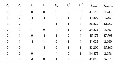
In this case, a parameter design experiment was carried out to adjust the width of the painted strip of a car painting system to a nominal width of 40,0 [cm]. The design of the experiment consisted of an orthogonal array L₉(3⁴) for the four control factors and a L₄(2³) for the three noise factors. Table 1 shows the control factors and their levels. More details and the data may be found in ^{Vandenbrande (2000}, 1998), and also see the appendix.

Table 1 Control factors and levels for the single-response real system 

Source: Authors

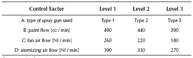
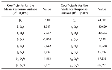
As can be seen from Table 1, factor A is a qualitative variable, whereas the rest are quantitative. Thus, Equations (7) and (8) must be used for estimating the model. In general, the model needs l - 1 dummy variables for representing a qualitative variable that has l levels (Myers & Montgomery, 2002). Given that factor A has three levels, the model must use two dummy variables for representing it. Since the design of the experiment consisted of an orthogonal array L9(34) for the four control factors, the study has nine data points for the mean and variance of the response. Thus, in order to leave one degree of freedom for the error term, the experimenter must choose only eight parameters to estimate. In this case, it was decided to estimate the position parameter and the four first order coefficients. Then, by examining the fit of the model to the data, the researchers began to include some quadratic terms, concluding that a good fit was obtained when considering the quadratic terms for factors B and C. With those considerations, the final models are the following:

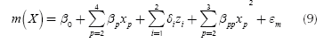
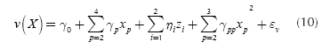
Table 2 shows the values of the coefficients of Expressions (9) and (10). ^_β0 and ^_γ0 are the position parameters. The variables ^_z1 and ^_z2 are the two dummy variables representing factor A, x₂, ^_x3 and ^_x4 represent the first order coefficient for factors B, C and D and, ^_x22 and ^_x32 represent the quadratic coefficients for factors B and C. Note that variables x₂, ^{_{x3, x4}} were rescaled and centered on their means, so that the values of them lie between -1 and 1 (per the procedure suggested in Myers & Montgomery, 2002). The models as well as the coefficients are all statistically significant at least at the 0,05 level. The ^_R2 for the mean response surface is 0,899 and 0,987 for the variance surface. Thus, it can be said that the response surfaces are a good representation of the true system.

Table 2 Regression coefficients for the mean and variance response surfaces 

Source: Authors

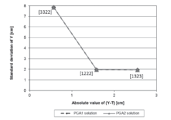
The two response surfaces were used in PGA2 to find an approximation to the Pareto frontier and 30 experimental runs were performed. Figure 1 shows the Pareto efficient solutions that were found by PGA2 (marked with a square), along with the ones delivered by PGA1 (marked with a rhomb). In Figure 1, the values shown in square brackets indicate the levels of factors set in each solution. For example, solution [1222], represents control factor A = 1 (spray gun Type 1), B = 2 (paint flow of 440 [cc / min]), C = 2 (fan air flow of 220 [Nl / min] and D = 2 (atomizing air flow of 330 [Nl / min]). The horizontal axis shows the mean adjustment as |y - T| attained by each solution in [cm]. The vertical axis shows variability reduction as s (standard deviation) of the response in [cm]. Note that the solutions delivered by PGA1 and PGA2 define similar Pareto frontiers. All of the solutions were consistently found in the 30 runs. Thus, for this case, PGA1 and PGA2 have a similar performance. Given that this single-response system has a few control and noise factors and is quite simple, a more refined missing value estimation mechanism does not impact too much the performance of the PGAs. Also, and as expected, since the surfaces that represent the mean and variance of the system are a good approximation to the real system, PGA2 has a good performance. In the next subsection, we test PGA2 under less favorable conditions, so that we can show how much PGA2's performance is reduced.

Source: Authors

Figure 1 Pareto frontier for the solutions corresponding to the real single-response system. 

Results obtained for the single-response complex systems

To test both PGAs under a more complex situation, a simulator was built, which is described in detail in ^{Canessa, Droop & Allende (2011)}. The robust design for this situation considers using an inner array L₆₄(4¹⁰) for the ten control factors and an outer array L₁₆(4⁵) for the five noise factors, which represents a hard to treat system (^{Taguchi, 1991}; ^{Roy, 2001}). For the following case studies, the four responses of the simulator are optimized independent from each other, so that both PGAs deal with four single-response systems.

Since there are four single-response systems with ten control factors and five noise factors, it would take many pages to describe all the details and present all the figures of the building of the four response surfaces (see the appendix for further important details). Thus, here we present only the most relevant aspects of that procedure. Readers interested in further details may contact the corresponding author. The experimental design considered factors with four levels each and a total of 1024 design points (64 treatment combinations for control factors times 16 treatment combinations for the noise factors). Given that the inner array has 64 treatment combinations, the experimenter can estimate up to 63 parameters, leaving one degree of freedom for the error term. However, when the experimenters were estimating the parameters, the multicollinearity statistics showed that such a problem existed. Thus, they looked at the VIF of each coefficient and began an elimination process for the variables that might have caused that problem, arriving at the models for the mean and variance of each of the four responses shown by Equations (11) and (12), which are versions of Expressions (5) and (6) since all the ten control factors are quantitative variables:

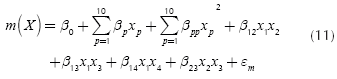
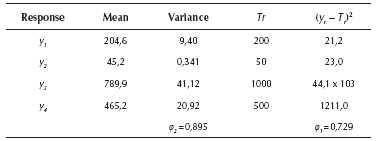
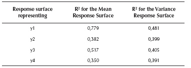
Expressions (11) and (12) show that the experimenters estimated the position parameter, all the linear and quadratic coefficients and the interaction terms corresponding to double interactions AB, AC, AD and BC (see the appendix for further details). Later, for corroborating whether those models were a good approximation to the true response surfaces, the estimated models and coefficients were compared to the expressions that comprise the simulator. The expressions and coefficients of the simulator may be seen in ^{Allende, Bravo & Canessa (2010}) and the comparison showed a modest approximation. Table 3 presents the ^_R2 for each of the four response surfaces corresponding to the mean and variance of each of the system's outputs. The ^_R2 are rather good, considering that the simulator was deliberately set with a large Gaussian noise, especially for response ^_y4, which causes that response surface ^_y4 to have the smallest ^_R2 among the four response surfaces. To be on the safe side, we added a large noise because we wanted to assess the performance of RSM and PGA2 under unfavorable conditions. Given that for the real system the ^_R2 values are high (0,899 and 0.987) and PGA2 works very well, we thought that it would be appropriate to test PGA2 under less favorable conditions. Hence, if the method works under those adverse conditions, it should perform even better in more favorable situations, as the results for the real system show.

Table 3 R² for each of the estimated mean and variance response surfaces 

Source: Authors

After estimating the response surfaces, these were used in PGA2 and 30 runs were executed for finding solutions. The next paragraphs present the results for each of the four responses.

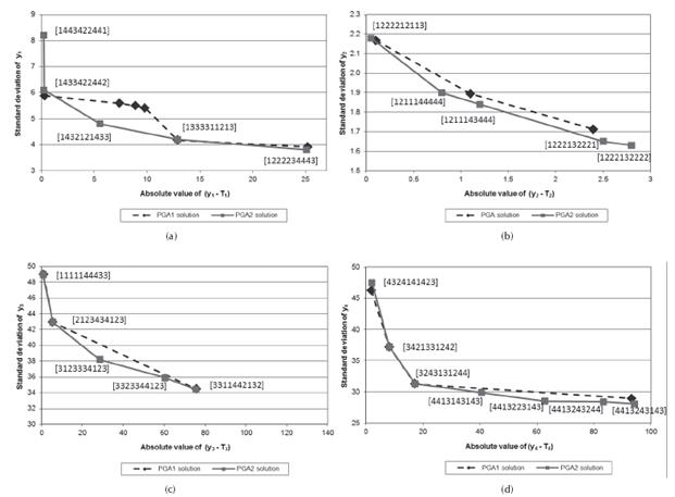
Figure 2 presents the solutions corresponding to the Pareto frontier found by PGA2 for the four single-response systems (marked with a square). Those solutions were consistently found in the 30 runs performed. Also, Figure 2 shows the solutions delivered by PGA1 in a previous study (^{Canessa et al., 2014}), marked by a rhomb. The horizontal axis shows the mean adjustment as |y_r - T_r | attained by each solution for response r. The vertical axis shows variability reduction as ^_sr (standard deviation) for each response r.

Source: Authors

Figure 2 Pareto frontier for the solutions corresponding to the single-response system: (a) y₁ (b) y₂ (c) y₃ (d) y₄. 

For response y₁, Figure 2 (a) indicates that PGA2 delivered five solutions, whereas PGA1 found 6 points. However, note that the Pareto frontier defined by PGA2 is better than the one obtained by PGA1. PGA2's Pareto frontier is totally convex, while the one of PGA1 is not. Also, the Pareto frontier delivered by PGA2 is a better approximation to the real unknown Pareto frontier, given that PGA2's solutions define a Pareto frontier that is closer to the optimal point of mean adjustment and variability reduction, i.e. |y₁ - T₁| = 0 and ^_s1 = 0, than the one obtained by PGA1. Thus, we can say that the missing value RSM estimation method improved the performance of PGA2 for response ^_y1. For further details regarding the assessment of performance see the appendix.

For response y₂, Figure 2 (b) shows that PGA2 found five efficient solutions, whereas PGA1 found only three. As before, PGA2's solutions define a better approximation to the Pareto frontier and PGA2 also found two more extreme solutions ([1222132221] and [1222132222]).

Regarding response y₃, PGA2 and PGA1 found almost the same solutions in terms of mean adjustment and variability reduction. However, PGA2 delivered one additional solution [3123334123] that helps better define the Pareto frontier. Note that solution [3123334123] shifts down-left the Pareto frontier, which strictly speaking, removes solution [3323344123] from the frontier. Given that PGA2 delivered solution [3323344123] as a Pareto efficient one, the Pareto frontier is not totally convex. However, the approximation is good.

Finally, for response y₄, Figure 2 (d) shows that two solutions obtained by PGA2 are exactly the same, in terms of |y₄ - T₄| and ^_s4, as the ones found by PGA1 ([3421331242] and [3243131244]). Also, two other solutions are very similar ([4324141423] and [4413243143]). Additionally, PGA2 found three new solutions that define a somewhat better Pareto frontier than the one delineated by PGA1. Although PGA2's frontier is not totally convex, the approximation is very good.

In summary, for the four single-response systems, the RSM-based missing value estimation method improves the performance of PGA2 compared with PGA1. Note that although the response surfaces are modest approximations to the real outputs of each system, still the new method attains good results. Recall that we deliberately added a large noise to the responses. Given that the method works rather well, we believe it should perform even better in more favorable situations.

Results obtained for the multi-response complex system

This case study used the same simulator and the same experimental design as before, but it optimized the four responses at the same time. This means that the PGAs are optimizing a four-dimensional multi-response system. The estimation of the response surfaces for PGA2 is the same as the one already presented for the four single-response systems, i.e. the estimation procedure is the same for univariate and multivariate systems.

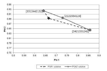
As in the previous analysis, 30 runs for PGA1 (see ^{Canessa et al., 2014}) and PGA2 were carried out. Figure 3 presents the solutions found by both PGAs. Note that in this case, the horizontal axis of Figure 3 shows the desirability function value ^_φ1 corresponding to mean adjustment and the vertical axis presents the desirability function ^_φ2 representing variance reduction. Remember that a larger value of ^_φ1 means a better mean adjustment and a larger value of ^_φ2 represents a smaller variance, so that the PGAs must maximize ^_φ1 and ^_φ2 (see Equation (4) and the appendix).

Source: Authors

Figure 3 Pareto frontier for the solutions corresponding to the multi-response system. 

From Figure 3, one can see that both PGAs found three solutions. These solutions were consistently found in all 30 runs performed. Of them two are similar (solutions [3312442132] and [3421331242]) and one is a different solution ([2122334124] of PGA2). This solution of PGA2 defines a better approximation to the Pareto frontier. Given that the PGAs are dealing with a maximization problem, the frontiers should be concave, which is the case for the frontier defined by PGA2's solutions, whereas the one for PGA1 is not totally concave. Furthermore, since the Pareto frontier delivered by PGA2 is closer to the upper-right corner of the graph, which corresponds to the optimal point ^_φ1 = ^_φ2 = 1,0, this frontier is a closer approximation to the real unknown Pareto frontier.

Note also that although the response surfaces are a modest approximation to the real mean and variance surfaces of the outputs of the system, given the large noise deliberately added to the responses (see Table 3, ^_R2 of surfaces between 0,5 and 0,35, except for the surface of the mean of ^_y1 with ^_R2 equal to 0,8, to which we added a small noise), the missing value estimation process based on RSM works rather well, enhancing the capability of PGA2 of finding a good approximation to the Pareto frontier. Hence, we should expect that under more favorable noise conditions, PGA2 should work even better.