Angular Position Measurement

The basic configuration of a system to control the angular position of a motor requires, in addition to the controller, three components: a driver, the motor, and a sensor. The driver uses two operational LM386 amplifiers set as a bridge to allow the motor to rotate clockwise or counter clockwise. The actuating signal coming from the controller feeds the amplifier card, so that, in the steady state, the motor rotates at a speed proportional to the actuating signal.

There is a huge variety of sensors used to measure the angular position of a motor. The usual selection is an incremental encoder, but other popular choices are the absolute optical encoder and the resolver. Applications with low precision requirements, as well as small angle variations, can be measured using potentiometers. Given the high cost of an absolute encoder or a resolver, the low precision of a potentiometer, and the undesirable dependency on the initial conditions of an incremental encoder, this paper presents the design of a sensor based on the Hall effect. This sensor aims to be absolute, as well as cheap and precise.

The sensor has two components: one rotates while the other remains still. The static part has two Hall effect sensors in quadrature, plus the electronic to normalize the signal. The rotating part uses two magnets in the shaft, which produces sine and cosine type output signals in the sensors, as described in (^{Rapos, Mechefske, and Timusk, 2016}), which is the configuration used in this paper. However, there are other interesting proposals to explore in future applications. For instance, ^{Wu and Wang (2016)} use three or six hall sensors instead of two to improve accuracy at the expense of increasing the complexity of signal processing. On the other hand, ^{Anoop and George (2013)} use two hall sensors, but propose the use of linear outputs instead of sinusoidal outputs, which may boost measurement accuracy.

The signal conditioning component shown in Figure 1 starts by filtering the noise that may appear due to mechanical vibrations or electrical interferences. The implementation of this filtering uses a traditional low-pass filter of the first order out fin = 1/(st +1), which can be written using a discrete set of blocks in Simulink, following the rule out = (1/s) (1 /t) (in - out). This configuration allows the definition of an initial output for the filter as the initial condition of the Integrator (1/s). That initial condition equals the initial measurement in each sensor, whereas the subtraction in - out corresponds to a negative feedback connection, which passes through the constant 1 /t in order to define the cut frequency of the filter (r = 2 ms). On the other hand, the constants in the signal conditioning section in Figure 1 serve to set the average signal to zero and the amplitude to one. These values were experimentally set at c₁ = 1,094, c₂ = 1,0144, c₃ = 0,277, c₄ = 0,664. This normalization facilitates the computation of the angle made by means of a atan2 function. This function uses x and y to come up with and angle between ±n, instead of the traditional ±∏/2 with the function atan.

Source: Authors

Figure 1 Block diagram of the angle estimation. 

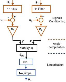
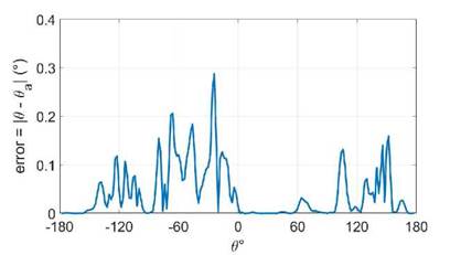
Any mechanical misalignment in the measurement configuration or between the sensor gains causes a discrepancy between the actual angle, θ, and the output of the function atan2, also called θ _m . This difference was as high as 10%, so the author used a neural network (NN) to reduce that error. The basic idea to reduce the error is to train a NN to learn the inverse relationship between θ and θ _m . Thus, when a mechanical position 9 produces an estimation equal to θ _m , that estimation ideally produces an output equal to θ in the NN. The author used a feed-forward backpropagation network with 8 neurons in the input layer and 4 neurons in the hidden layer. The input data θ cover angles between -180° and 180°, with data points every 1°. Figure 2 shows the error in the estimation using the NN to linearize the angle measurement. The error always remains under 0,3^°.

Source: Authors

Figure 2 Error in the angle estimation. 

The estimation of the angle covers a single turn from -180° to 180^°. Going further means generating discontinuities in the approximation due to the behavior of the function atan2. The final step in angle approximation implies avoiding those discontinuities, as depicted in Figure 1 by the block "No jumps". The author starts by using two new variables to detect the discontinuities: cd for jumps from 180° to -180°, and cu in the other case. Those constants start at zero and increase by one every time the difference between the current and the previous angle goes under -300° for cd, or over 300° for cu. The value ±300° was defined experimentally under the consideration that it should be higher than the delta angle produced at the maximum speed between two consecutive angle samples. Thus, the final approximation can be written as θ _α ← 360(cd - cu) + θ _α .

System Identification

The plant in this application is a permanent magnet direct current motor (PMDC) with a nominal current of 500 mA and nominal voltage of 12 V. This motor is widely used in robotics and it is the most popular option to test control algorithms. However, its parameters are unknown to the author. We could apply some tests to approximate the parameters of the motor, but we preferred to use the approach in this section. Firstly, because those parameters assume a linear system, when they do not; the motor can be seen as linear only around the nominal values of current, voltage, speed, and temperature. Secondly, the process used in this paper requires a single set of data to capture a model that resembles the whole dynamic instead of running several tests to obtain a model.

Atraditional DC motor model uses linear differential equations to represent the relationship between the states in the motor. In this linear model, the input voltage produces an electrical current which generates a mechanical torque resulting in the rotation of the motor. Identification, in addition to the equations, requires the computation of electrical, electromechanical, and mechanical constants, such as resistance, inductance, the constant of friction, and the constant of inertia, as is presented in ^{Wahyunggoro and Saad (2010)}. This type of model is used to study the motor as a dynamic system. It can also be part of a first attempt to design a controller. However the approximation given by a set of linear equations cannot fully emulate the richness of the dynamic in a real machine.

Instead of a pure linear model, ^{Aquino and Velez (2006)} propose a gray-box model. In this model, the electrical part is linear and known, whereas the mechanical part is nonlinear and unknown, as a result of the effect of changes in the load. The author proposes the use of Radial Basis Neural Networks to capture the nonlinear behavior of the model, and compare the results using a recursive two-stage method. Another approach in the identification assumes that the whole model is unknown. Thus, the linear part of the model can be represented by an ARX model, whereas the nonlinear part is chosen to be a polynomial of known order, as presented in ^{Kara and Eker (2004)}. These authors study the effect of nonlinear friction and other nonlinearities in the model under the assumption that it is possible to separate the nonlinearities in two groups: static and dynamic. Another proposal by ^{Rios and Makableh (2011)} uses a Feed Forward Neural Network to capture the nonlinearities of the motor. That model is then used to simulate the effect of another neural network working as a controller of the motor. This last proposal focuses on two of the main nonlinearities studied in this paper: dead zone and saturation.

The identification of the motor in this paper uses some characteristics of the proposals in the references above, but instead of looking for a very accurate model, this paper shows that a model that approximately captures the main features of the dynamic is enough to get good control performances using time scaling. The core of the model presented in Figure 3 emulates the transient behavior of the motor using two linear blocks: one for the relation between the input voltage and the speed in the shaft (a second order transfer function, H(s)), and the other for the relation between speed and angular position (an Integrator, 1fs). Given the author' experience controlling the motor, there are two main nonlinearities that should be included in its model: 1) the dead zone, and 2) the gain of the steady-state as a function of the rotation sense. The dead zone is represented by the first block in Figure 3, while the gains correspond to the triangles. The model includes another nonlinearity, the saturation of the Integrator, in other words, the natural limits for the rotation of the motor. The block between the gains and the Integrator symbolizes the selection of one gain or the other depending on the sense of rotation. If the speed is greater than or equal to zero, then the gain for the model is k _ccw ; if the speed is negative, the gain is k _cw .

Source: Authors

Figure 3 Motor model scheme. 

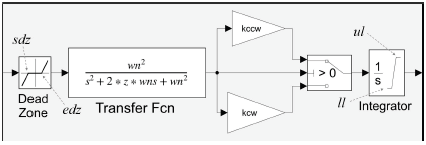
This is the list of parameters for the model, according to the model in Figure 3:

The computation of these parameters starts by defining the last two: ul and II. Even when the control rank equals ±90°, the limits are greater than that rank. A first extra 10° allows the human controller to make mistakes at the ends of the rank and still generate good data to train the controller. A second extra 10° bounds the parameter estimation algorithm to vary the parameters of the model. Thus, the control rank is ±90°, but the human control covers +100°, while the estimation algorithm has a window of ±110°. Thus, ul = 110° and II = -110°. The next two parameters correspond to the transfer function H(s) in the block "Transfer Fcn". These two parameters define the shape of the transient when the input of the model changes. A way to evaluate these values implies generating sudden changes in the input of the motor and then measuring the speed of the shaft. The values that match those transients better are rounded to w _n = 100 rad/s, and ζ = 1.

The four remaining parameters of the model were computed using the tool Parameter Estimation of Simulink. Given that the main goal of the model is to emulate the system when the controller is working, then a proportional controller with kp = 1/10 leads the motor during the acquisition of the input and output data. The whole experiment lasts a minute and uses samples every millisecond, so there are 60001 data points for the input and the same number for the output. The reference for the control system is a step function randomly changing from 0,3 to 0,7 s with also random amplitude from -100° to 100°. This signal was smoothed using a first order filter with constant time of 0,1 s, which better emulates the work of the motor during normal conditions. The optimization method is the Nonlinear Least Squares and the algorithm is Levenberg-Marquardt. The tolerance in the optimization is 0,001. Afinal estimation was run, including all the parameters except the saturation constants. The natural frequency changes to w _n = 300 rad/s. It is important to report that the change from 100 to 300 in w _n didn't alter the quality of the approximation in more than 0,1%, which means that the nonlinearities affect the dynamic of the motor more than the linear part. The results of the optimization are shown in Figure 4, where the lower part corresponds to the input voltage, while the upper part is the output of the plant and the model.

Source: Authors

Figure 4 Output data and simulated output under the same input. 

A traditional modelling process for a DC motor defines the model as a linear transfer function, and that approximation may be useful when working around the nominal conditions of the machine. However, the DC motor for this application changes the nominal speed depending on the rotation sense, as expressed by means of the gains k _cw and k _ccw . These gains can be evaluated as the quotient between the speed in °/s at nominal voltage in V, for both positive and negative cases of voltage, but, in this case, Simulink made the approximation based on the data in Figure 4. The result is that k _cw = 940° /s/V whereas k _ccw = 530° /s/V. Thus, the motor is almost two times faster in a clockwise sense than in the counter clockwise sense.

The last two constants of the model express the fact that the voltage in the motor requires to pass a certain threshold before the shaft starts to rotate, mainly given the friction effect. An initial estimation of those constants can be made by increasing the voltage to the point that the shaft starts to rotate, but, once more, that approximation was made by Simulink based on the data in Figure 4. The rotation sense changes the threshold, so the model requires the estimation of that value in both senses, as defined by using the gains sdz and edz inside the block "Dead Zone". The values for those gains are sdz = -0,9 V and edz = 0,6 V.

In summary, the model in Figure 3 has dead zone sdz = -0,9, edz = 0,6; transient w _n = 300, ζ = 1; gains k _cw = 940, k _ccw = 530; and saturation: ul = 110°, II = -110°.

Scaling Stage (S)

The model in Figure 3 uses the traditional definition of time, but that dynamic is too fast for a human to control. Thus, this section starts by scaling the linear components of the motor, as defined in Equation (1), according to the presentation in ^{Rairán (2017)}. It can be seen that the nonlinear components are not time-dependent, but constant, so the nonlinear part remains equal regardless of the time scale. The constant k _t in Equation (1) corresponds to the scaling factor. For instance, k _t = 5 means that the new dynamic H' is five times faster than the dynamic H. The new plant, H', keeps amplitude and shape of H and only changes how long a transient lasts.

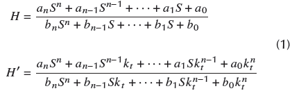
Defining the scaling factor implies an experimental procedure where the human controlling the system changes that factor until achieving a value that makes control of the system comfortable. In this case, this value is set to k _t = 1 /30, which means that the scaled system is 30 times slower than the original. In this way, for instance, a transient of two seconds in the motor lasts a whole minute in the scaled model. The transient H = 300²/(s ² + 600s + 300²)) corresponds to H' = 100/( s ² + 20s +100), and the integral θ(s)/Vel(s) = 1/s corresponds to θ'(s)/Vel'(s) = (1/30)/s. Both input and output in each transfer function need to be scaled as indicated by the notation. The slow human reactions produce a slow velocity, which in turn produces a slow change in the angular position. The scaling additionally requires the scaling of the sampling time at which the data is recorded or generated, from t _s to t' _s = t _s /k _t in this case, t _s = 1 ms, so t' _s ^' =30 ms.

This stage in the control process requires interaction between the human and the scaled system. The human senses and evaluates the behavior of the plant, and, with experience in the manipulation of the system, compares his or her perceptions with the set point. As a result, the human makes two decisions: 1) whether to increase, decrease or maintain the actuating signal, and 2) how significant this change will be. The application of the actuating signal as input for the scaled system produces changes in the output of the scaled plant in such a way that, ideally, the perceived output matches the set point in the shortest time possible. The instantiation of the control stage in this paper uses a computer and a human, as shown in Figure 5.

Source: Authors

Figure 5 Control Scheme. 

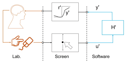
This stage aims to generate the best data to train a NN in the next stage. Thus, the definition of the reference signal should make the system as dynamic as possible. In this case, the author defines a square signal oscillating between 100° and -100°, lasting between 12 and 15 seconds in each value. That signal passes through a low pass filter of the first order with τ = 2 s, as shown in Figure 6. This filter produces references along the rank of ±100°, instead of the extreme values alone. The constant time τ aims to emulate the normal work of the motor during a traditional control application, and at the same time its stabilization time falls just below the transition time, which allows the system to reach its steady state. The data acquisition lasts 2,5 minutes. Thus, every reference value appears about five times, which is enough data to train a NN.

Source: Authors

Figure 6 Control system in Simulink. 

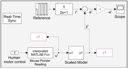
Figure 6 also shows that the information presented to the human controller through the scope is not the scaled error, e' (as it is done in traditional control), but its negative, -e'. It can be seen that, regardless of the value of the output y', the output will eventually match the sign of the input u'. For instance, if u' increases, then y' (as well as -e' = y' - r') will eventually also increase. Thus, if -e' is, for instance, negative, a good control action will consist of setting u' as a positive value. This action is intuitive for a human: it is performed to counteract the signal in the screen in order to have null error. On the other hand, the block "Mouse Pointer Reading" in Figure 6 runs a function based on the function "gpos" of Matlab, which provides the coordinates of the pointer of the mouse. The y value of the pointer corresponds to the value of u' ^' .

Blocks u1 and y1 in Figure 6 save the data generated during the running of the simulation and make it available for use in the workspace of Matlab. The signal u' corresponds to the actions of the human controller, while y' provides the corresponding emulated position given by the scaled model. Finally, the block "Real-Time Sync" allows the running of the simulation in real time using the Simulink Desktop Real-Time toolbox.

Training Stage (T)

This stage uses the data coming from the previous stage to train a NN. Thus, instead of the human controlling the motor, the system uses the NN to define the actuating signal. The training stage starts by normalizing the data, which implies cutting and scaling. By cutting, the author understands triming and deleting the first 15 seconds of the experiment, given that this is the time required for a person to accommodate, concentrate, and be focused on the control problem. The scaling consists in dividing the input e by 180, as shown in Figure 7. This scaling makes the rank of the input [-1.1, 1.1], which is close to the rank of the activation function of each neuron [-1, 1]. Nevertheless, the effectiveness of the training remains equal under the scaling or without it in this application. The scaling makes a difference when looking at multiple inputs, as could be the case of future work, when the problem requires (for instance, in addition to e', its derivative). Normalization makes all the inputs have a similar influence during the training.

Source: Authors

Figure 7 Effect of the number of neurons in the training. 

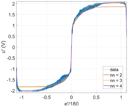
An analysis of the sorted data in Figure 7 shows the relationship between the error and the actuating signal. That relation looks like a tangent sigmoid function. This observation favors the use of a Multilayer Perceptron Neural Network to learn the given data, so that each of its neurons may have a tangent sigmoid transfer function. It can be seen that sorting error evinces the control strategy of the human, which was hidden inside the brain of the human controller until now. It is possible to divide that strategy in three zones: 1) small errors, from 0 to 0,2; 2) medium errors, from 0,2 to 0,8; 3) major errors, from 0,8 to 1,1. Zone 1 presents the highest rate of change and happens where the majority of control takes place. Zone 2 has a smaller slope and resembles the saturation of a tangent sigmoid. Zone 3, contrary to the intuition, decreases the actuating signal. This last behavior is caused by the reaction time of a human due to large errors (positive or negative). Unlike a pure mathematical algorithm, the control interface (including the brain itself) does not allow the human to change a decision instantly. However, a positive aspect of that delay is that it reduces the overshoot in the response.

The author used the Levenberg-Marquardt algorithm to train the NN, with a maximum of 1 000 epochs, and data randomly divided into three sets: 70% to train, 15% to validate the training, and 15% to test the NN. Figure 7 shows the result of changing one of the most influential parameters during the learning process: the number of neurons in the network.

Results in Figure 7 regard networks with a single hidden layer with two, three, or four neurons. Two neurons miss the third zone. Three neurons resulted better than two, but the generalization for major and negative errors fails. The best result in Figure 7 uses four neurons. That network properly matches and generalizes the data across the three zones.

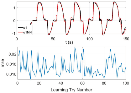
Figure 8 shows the results when training 100 neural networks with four neurons in the hidden layer. The lower part of the figure shows the final mean square error mse for each training. This error was used as the measure of quality during the learning process. It can be seen that the variation of mse is not big: the best mse is 0,015, while the worst is 0,022. The upper part of Figure 8 presents the results for the NN with the best performance out of the 100 trials. This part of the figure shows the output data u1 and the output of the network (u1NN) when fed with the same input. The network closely follows human control behavior, especially in Zones 2 and 3.

Source: Authors

Figure 8 Selection of the best neural network. 

Running Stage (R)

This final time scaling control stage uses the best Neural Network of the previous stage. The best network defines an actuating signal based on the error value in order to control the models and the motor itself. The same network can control models and motor since the Multilayer Perceptron Neural Network is blind to changes in the scale of time. This type of NN produces the same outputs if the same inputs are given, regardless of time variation. If an input changes, the corresponding output is updated after a few mathematical operations. These operations are instantaneous in practice, given the speed of the systems in contrast with the time it takes to propagate a network. Thus, the same network controls the simulated system and the real plant.

Testing the trained NN starts with running the control over the scaled model H' because the controller was trained using data from H'. The test during the scaling stage lasts 2,5 minutes, which is enough time to train the network. However, the simulation in this stage may last longer, that is, 30 minutes or more. It can be seen that there is no risk that the network will stop paying attention, as it actually happens with humans after a few minutes. In addition, instead of two unique values +100°, it is better to test several and random amplitudes in the rank ±90°. If the control works properly, the next step in testing consists of using the same network over system H. This last simulation could take a single minute, because the system runs at its normal speed (remember that a minute at the unscaled time corresponds to 30 minutes using the scaled time, kt = 1/30). Thus, the transitions between one amplitude and another may last from 0,3 s to 0,6 s. If this test succeeds, it is possible to run the final test, which is to control the real plant. If not, the Training stage should be run again.

The final and definite test uses the trained NN to control the real plant. The block diagram of the connections inside the computer is shown in Figure 9. It can be seen that the input of the network is scaled dividing the error by 180. The output of the controller reaches the plant using a data acquisition card, the National Instruments PCI-6024E. This card translates the actuating signal inside the computer into voltage to feed the power amplifier that drives the motor. Figure 9 also shows a traditional PID controller with the same tuning that was used during the Scaling stage, it is a proportional controller with k _p = 1/10.

Source: Authors

Figure 9 Block diagram to control the real plant. 

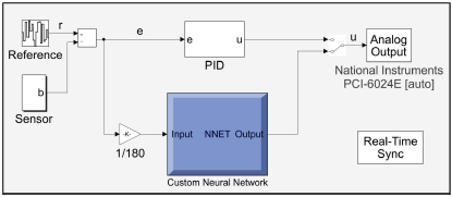
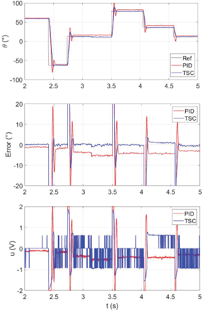
Figure 10 shows the performance of the Time Scaling Controller during the control of the real plant. The upper part of the figure presents the reference, the output with a PID controller, and the output with the proposed controller in this paper. TSC presents a lower overshoot and reaches the reference better, as can also be seen in the middle figure. It has a null error for the steady state after almost all the transients, but the PID has a steady state error of about 4^°, this is due to the effect of the dead zone. The lower part of Figure 10 shows the actuating signal for both controllers. It is important to remark that TSC does not reach the limits of ±2, but the PID controller does it. This characteristic reveals that the trained NN uses the energy to control the plant better than the PID for the experiment in the figure. The switching of the actuating signal for TSC happens because the controller reaches null error, so that the signal jumps alternatively from negative (or positive) to a null value. The actuating signal for the PID does not switch because it almost never reaches the null error. Finally, a measure of the performance for both controllers is the index Integral of the Absolute Error (IAE). For a trial of ten seconds, the result for the PID is 56,8 and 37,8 for TSC. Thus, the ratio between the two controllers is about 1,5 in favor of the Time Scaling Controller.

Source: Authors

Figure 10 Control performance comparison.