


 English (pdf)
 Article in xml format
 Article references
 Send this article by e-mail
 Cited by SciELO
  Cited by Google
  Similars in
SciELO
Similars in
SciELO  Similars in Google
 Permalink
Introduction
Genetic algorithms (GAs) are random-based evolutionary methods. They are preferred over classical optimization due to their versatility in solving complex problems and finding multiple solutions without a priori information (Deb, 1999). They are inspired by fundamental genetic laws such as natural selection, first introduced by Fraser (1957), and further popularized by Holland (1975). When we study GAs, we contemplate an initial population of pseudorandom solutions that pass through genetic functions such as selection, crossover, and mutation to recombine and perturb solutions. Then, we evaluate these solutions with a fitness function in the hope of creating the fittest ones that will survive and evolve to the next generation. Finally, this process ends when we use a predefined termination criterion.
GAs then evolved to Multi-Objective and Many-objective Evolutionary Algorithms (MOEAs and MaOEAs) to optimize Multi-Objective or Many-Objective Optimization Problems (MOOPs and MaOPs) for fields such as engineering, business, mathematics, and physics (Li, Wang, Zhang, and Ishibuchi, 2018). They search for multiple solutions simultaneously on different non-convex and discontinuous regions next to the approximated Pareto front. Initially, research focused on solving MOOPs, but recently, there is an increasing interest in solving MaOPS. However, for MaOPs, we have a significant number of non-dominated solutions that exponentially increase with the number of objective functions. This is due to the selection operator and the dominant resistance caused by the dimensionality curse (Purshouse and Fleming, 2007).
The practical motivation of this paper is the implementation of an open-source version of the proprietary NSGA-III (Deb and Jain, 2014; Jain and Deb, 2014) called the EF1-NSGA-III (Ariza, 2019) that alleviates the above-mentioned issue of dimensionality. This algorithm solves problems with more than two objective functions, checks the feasibility of the population to fill the non-dominated sort procedure, and then uses the first front to generate non-negative and non-repeated extreme points during the normalization procedure. It has already been employed to reduce the power consumption for Cloud Radio Access Networks (Ariza, 2020), and resolve the Bi-Objective Minimum Diameter-Cost Spanning Tree problem (Prakash, Patvardhan, and Srivastav, 2020). The authors who solved the latter used the EF1-NSGA-III as a basis to generate a new algorithm called the Permutation-code NSGA-III (P-NSGA-III).
The EF1-NSGA-III uses a non-parametric method for diversity and executes faster when we take the renowned and efficient NSGA-II code, with prominent features such as simplicity, and an elitist approach. This algorithm, found at the repository of the Kanpur Genetic Algorithms Laboratory (KanGAL, 2011), is the core of the EF1-NSGA-III, but with significant changes to the selection operator. Our strategy for this paper is borrowed from professor Kalyanmoy Deb and researchers at Michigan State University. It helped them create and unify the NSGA-III to solve any mono-objective, multi-objective, and many-objective problem (Seada and Deb, 2015).
After we finished the extension of the EF1-NSGA-III, we continued with the adaptive EF1-NSGA-III (A-EF1-NSGA-III), and the efficient adaptive EF1-NSGA-III (A2-EF1-NSGA-III), which use different schemes of adaptive reference points to increase their associated number of population members and accomplish a better distribution of solutions. The last two new algorithms are inspired by the A-NSGA-III and A2-NSGA-III. These algorithms have already been implemented by referenced authors (Jain and Deb, 2013). Also, we contribute to explain how to generate reference points using the Das and Dennis (1998), two-layer, and adaptive methods.
The above contributions are the smoothest way we found to create a robust algorithm, rather than starting from scratch, as did Yarpiz (Matlab) (2018), jMetal (Java) (2018), nsga3cpp (C+ + ) (Chiang, 2014), nsga3 (Python) (Marti, 2016), and PlatEMO (Matlab) (Tian, Cheng, Zhang, and Jin, 2017). Recently, a Multi-objective Optimization framework in python called pymoo was created, and its NSGA-III implementation is available (Blank and Deb, 2020). This implementation is employed to compare the NSGA-III and the EF1-NSGA-III in terms of some performance metrics.
In the remainder of this paper, we present a revision of related works. Then, we describe our extensions of the non-dominated sorting genetic algorithms EF1-NSGA-III, A-EF1-NSGA-III, and A2-NSGA-III. After that, we present a detailed performance evaluation using statistical analysis. Finally, we draw conclusions.
Related work
Many real-life problems are MaOPs, and a whole army of evolutionary algorithms (Seada, Abouhawwash, and Deb, 2017, 2018) is waiting to be utilized to solve them. For example, some representative algorithms are the MOEA/D (Zhang and Li, 2007), the knee point-based algorithm (KnEA) (Zhang, Tian, and Jin, 2015), the HypE (Bader and Zitzler, 2011), and the NSGA-III. They are based on decomposition, convergence enhancements, indicators, and reference points, respectively. Any evolutionary algorithm mentioned before or even another extension of them has the chance to be improved considering different stages such as the generation of the parents and offspring populations, as well as the use of novel genetic functions that recombine and perturb solutions, the information feedback of individuals from previous iterations (Wang and Tan, 2019), or the evaluation of population members (the fitness allocation method) that allow solutions passing to the next generation.
Some of the already implemented learning methods to improve evolutionary algorithms are also inspired by nature, but, in this case, they mimic a herd or colony's behavior. We can mention some swarm intelligence methods as examples, such as chaotic krill herds (Wang, G., Guo, Gandomi, Hao, and Wang, H., 2014), elephant herds (Li,, Wang, and Alavi,, 2020), bee colonies (Wang and Ji, 2017), monarch butterflies (Wang et al., 2019), and moth colonies (Wang, 2016). These methods simulate the clustering behavior of chaotic krills, elephants, and also other insect behaviors such as migration and phototaxis. These algorithms imitate how groups of animals cooperate and learn by themselves or use information from other members to do a specific task such as finding food. Some NP-hard problems that benefited from those improvements are scheduling, image, feature selection, detection, path planning, cyber-physical social system, texture discrimination, saliency detection, classification, object extraction, economic load dispatch, global numerical optimization, multi-objective optimization, knapsack problem, and fault diagnosis problems.
As can be seen, there are many options to improve evolutionary algorithms including the NSGA-III algorithm. Some new extensions of the NSGA-III algorithm have been developed since 2013. These are the A-NSGA-III and A2-NSGA-III, which allocate adaptive reference points to improve the distribution of solutions (Jain and Deb, 2013). Another example is the U-NSGA-III, which uses the NSGA-III as the basis for implementing a unified algorithm to solve problems with up to 15 objective functions (Seada and Deb, 2015). The 0-NSGA-III trades off the diversity and the convergence of problems with more than four objective functions focused on the improvement of the non-dominated sort procedure (Yuan, Xu, and Wang, 2014).
Other works are the EliteNSGA-III, which increases the accuracy and diversity of the NSGA-III by maintaining an elite population archive to preserve previously generated elite solutions that would probably be eliminated by the original NSGA-III (Ibrahim et al., 2016). The E-NSGA-III utilizes extreme solutions in the population generation module to improve the overall quality of solutions (Wangsom, Bouvry, and Lavangnananda, 2018). The IFM-NSGAIII solves large-scale problems, instead of the small-scale problems, as the NSGA-III does, and introduces information feedback to influence the offspring population (Gu and Wang, 2020). The P-NSGA-III that modifies the elitist framework of the NSGA-III uses preferred vectors to improve local search (Shu, Wang, W., and Wang, R., 2018). Also, the Permutation-coded NSGA-III encodes chromosomes as permutations of graph vertices (Prakash et al., 2020).
Two more developments are the set of NSGA-III SBXAM, NSGA-III SIAM, and NSGA-III UCAM algorithms, which use an adaptive mutation operator and evaluate simulated binary crossover (SBX), uniform crossover (UC), and single-point crossover (SI) operators in large-scale and online problems (Yi, Deb, Dong, Alavi, and Wang, 2018; Yi et al., 2020). Finally, there is the B-NSGA-III, which converts continuous NSGA-III into binary NSGA-III modifying the initialization, crossover, and mutation operators for band selection in cloud contaminated hyper-spectral images (Gupta and Nanda, 2019).
The EF1-NSGA-III, A-EF1-NSGA-III, and A2-EF1-NSGA-III algorithms
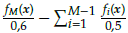
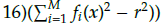
The basic framework of the proposed EF1-NSGA-III is similar to the KanGAL NSGA-II and inherits its parameters (Jain and Deb, 2013, 2014; Deb and Jain, 2014; Blank and Deb, 2020). It resolves MOOPs or MaOPs with conflicting objectives and inequality constraints focused on finding non-dominated solutions. Mathematically, the definition of the optimization problem is:
where x is a vector with p decision variables, M is the number of conflicting objectives, J is the number of inequality constraints, K is the number of equality constraints, and l is the number of bounds from low (L) to high (H).
We propose the EF1-NSGA-III, where individuals in the first front (F 1) are contemplated to obtain non-negative and non-repeated extreme points and guide the evolution of the algorithm. Algorithm 1 resumes the procedure.
The EF1-NSGA-III first checks if the remainder of N is divided by four to make systematic application pair-wise selection and pair-wise recombination operations (Seada and Deb, 2015). Then, it runs a finite number of generations defined in a loop by the user. In the beginning, the population P t is generated randomly, and its size is N (afterwards, the parent population comes from the last generation). Its offspring Q t is generated using tournament selection, mutation, and crossover operations, and its size is N. The combined parent and offspring population Rt = Pt + Qt has a size of 2N. Population R t is sorted according to different non-dominated sorting levels or fronts (F1,F2,F l ), where F l is the last front. All members of each front are selected one at a time to build Population St. If front members reach the size of the population Pt, there is nothing more to do for that generation and St = Pt+1. If St population plus the last front exceeds the size of Pt, then the last front F; is accepted partially, and l + 1 onward fronts are rejected. The last front F; selects members for population St that maximize its diversity through the niching operator. This operator requires the determination of reference points on a hyper-plane and adaptive normalization of population members, association operator until reaching the niching preservation operation. Finally, the next generation parent population Pt+1 is St, plus members from the niching operator, improve better the diversity until reaching the size N. There is no difference between the EF1-NSGA-III and the NSGA-III relay on normalization, niching procedures, and selection.
In the following section, we explain our implementations to generate reference points using simple algebraic principles. They are the well-known Das and Dennis, two-layer, k-layer, adaptive, and efficient adaptive methods (1998).
Das and Dennis approach
We used the Das and Dennis method (1998) for EF1-NSGA-III, A-EF1-NSGA-III, and A2-EF1-NSGA-III algorithms to generate well-distributed reference points and ensure diversity in obtained solutions. This method is the basis to generate different types of reference points such as two-layer, k-layer, adaptive, and efficient adaptive.
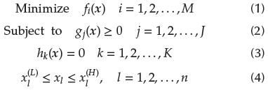
The predefined Das and Dennis approach places reference points on a normalized hyper-plane equally to all axis and has an intercept of one on each axis. If p divisions are considered along the M axis, the total number of reference points H is determined by
This reference point generator is used for problems with up to five objective functions. An example can be seen in Figure 1a, for M = 3 and p = 12. High-dimensional problems with more objective functions require a different approach because the number of reference points increases exponentially with the number of objective functions.
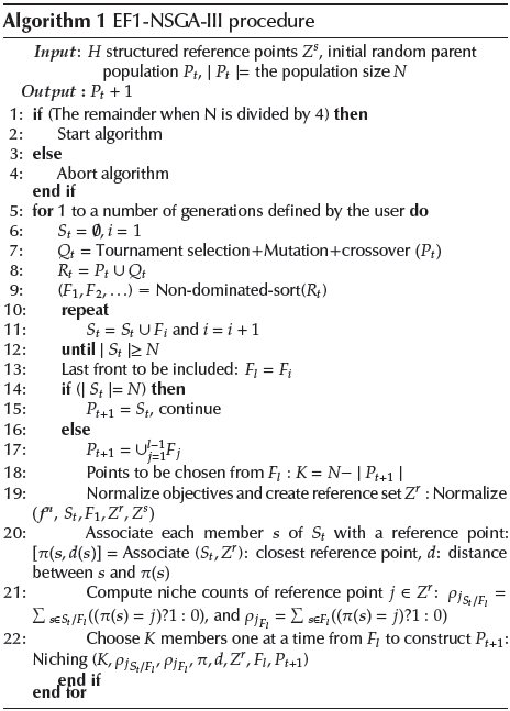
Two-layer of Reference Points
This alternative reduces the number of reference points for high-dimensional problems compared to the Das and Dennis method. This approach is divided into the following steps:
1. Generate reference points of the boundary layer: Use the Das and Dennis approach. The boundary layer must satisfy the plane equation x1 + x2 +…+ xnobj = 1, where nob j = M.
2. Generate reference points of the inside layer: Use the Das and Dennis approach again, but reference points of the inside layer should be on the plane x1 + x2 +…+ xnobj = 1-
 The number of divisions of the inside layer is ndiv -1, where ndiv = p.
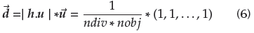
3. Move reference points from the inside layer to the boundary layer: Reference points of the inside layer are moved to the boundary layer by adding the value d =
 in all dimensions. Figure 1b, right side, depicts the distribution of reference points.
K-layer of Reference Points
It follows the two-layer reference points procedure, but with more than one inside layer. Additional information can be revised in Jiang and Yang (2017). Figure 1b, on the left side, shows the reference point distribution.
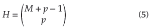
Adaptive Reference Points
First of all, this method requires the identification of useful or crowded reference points in cases where the niche count P jSt /Fl > 1(j Є {0,1,..., H -1}); and second, the generation of adaptive reference points around j th . Before a new adaptive reference point is accepted, it must be non-repeated and lie on the positive orthant. After the adding task, the niche value of all reference points is updated, and adaptive reference points with niche count P jSt/Fl = 0 are deleted. In the next generations, adaptive reference points are added and deleted as long as useful reference points exist. The procedure for each crowded reference point is described below:
1. Generate initial adaptive reference points for one division: Initial adaptive reference points x1 = ( ,0,...,0) x2 = (
,0,...,0) and x
nobj
= (0,0,...,
) are generated using the Das and Dennis approach to satisfy the plane equation x1 + x2 + … + x
nobj
=
,0,...,0) x2 = (
,0,...,0) and x
nobj
= (0,0,...,
) are generated using the Das and Dennis approach to satisfy the plane equation x1 + x2 + … + x
nobj
=
 .
.
2. Move adaptive reference points to the plane x1 + x2 + … + x
nobj
= 0: it is necessary to project the point p = (0,0,..., 0) onto the plane x1 +x2 + …+x
nobj
=
 . Any reference point of the plane can be chosen, for example, r =(
, 0,..., 0). With this vector in mind, vector h = p - r = (0,0,...,0) - (
,0,...,0) = (-
,0,...,0) is obtained. Immediately, the unit normal vector is
. Any reference point of the plane can be chosen, for example, r =(
, 0,..., 0). With this vector in mind, vector h = p - r = (0,0,...,0) - (
,0,...,0) = (-
,0,...,0) is obtained. Immediately, the unit normal vector is
 (1,1,..., 1). The vector to add initial adaptive reference points is:
3. Move adaptive reference points to the crowded reference point jth: In this step, after niching values P jst/Fl are updated, we identify crowded reference points with niche values P jst/Fl > 1. After that, we add to the adaptive reference point near the crowded reference point. In the end, for a three-dimensional case, the last three reference points create the inner triangle around each crowded reference point, as shown in Figure 1c on the left side.
4. Repeat previous tasks for all crowded reference points.
Efficient Adaptive Reference Points
This method has the following steps:
1. Generate efficient adaptive reference points for one division: Initial efficient adaptive reference points
 and
and
 are generated using the Das and Dennis approach (λ is a positive number called the scaling factor; its value is 1 for this work). They satisfy the plane equation x1 + x2 + … + x
nobj
=
are generated using the Das and Dennis approach (λ is a positive number called the scaling factor; its value is 1 for this work). They satisfy the plane equation x1 + x2 + … + x
nobj
=

2. Move efficient adaptive reference points to the plane x1 + x2 + … + x
nobj
= 0: Initial efficient adaptive reference points are moved a distance d =
 in all dimensions.
3. subtract efficient adaptive reference points: One of the previous efficient adaptive reference points is subtracted. In a three-dimensional case, this task is executed three-fold to obtain nine points (three of them are the same vector (0,0,0)).
4.
Move efficient adaptive reference points to the
crowded
reference point
jth: The final structure of reference points is moved next to the
crowded
reference point at a distance d =
in all axes. Considering a three-dimensional example, the efficient adaptive reference points create three triangles connected to the crowded reference point as depicted in Figure 1c on the right side.
5. Repeat for all crowded reference points.
In next subsections, we show the procedures for the EF1-NSGA-III, except the associate one that is the same as the one from the NSGA-III authors.
Normalization of Population Members
We normalized the objective values of population members to have the same range of the reference points as presented in Algorithm 2. The normalization procedure has the following steps:
First, we construct the ideal vector
 of the population S
t which is determined by identifying the minimum value from each objective function. Second, we translate each objective f
j
(x) by subtracting zmin
j
, denoted as f’
j
(x) = f
j
(x) - zmin
j
. Third, we determine M extreme points to constitute a M-dimensional hyper-plane that makes the Achievement Scalarization Function (ASF) minimum (Blank, Deb, and Roy, 2019), expressed as zj,max = f
m
(x) | minnЄF1 {ASF
j
} where j Є {1,2,...,M}, and n is the population size of the first front F1. The
ASF
j
function finds the maximum translated objective value divided by the scalarization value in all dimensions, denoted as
ASF
j = maxminM{f’
m
,(x)/sj
m}. For example, in a three-objective problem, we have the scalarization vector s1 = (1,Є,Є) for j = 1, s2 = (Є, 1, Є) for j = 2, s3 = (Є, Є, 1) for j = 3, where e is a small value such as 0,0000000001.
of the population S
t which is determined by identifying the minimum value from each objective function. Second, we translate each objective f
j
(x) by subtracting zmin
j
, denoted as f’
j
(x) = f
j
(x) - zmin
j
. Third, we determine M extreme points to constitute a M-dimensional hyper-plane that makes the Achievement Scalarization Function (ASF) minimum (Blank, Deb, and Roy, 2019), expressed as zj,max = f
m
(x) | minnЄF1 {ASF
j
} where j Є {1,2,...,M}, and n is the population size of the first front F1. The
ASF
j
function finds the maximum translated objective value divided by the scalarization value in all dimensions, denoted as
ASF
j = maxminM{f’
m
,(x)/sj
m}. For example, in a three-objective problem, we have the scalarization vector s1 = (1,Є,Є) for j = 1, s2 = (Є, 1, Є) for j = 2, s3 = (Є, Є, 1) for j = 3, where e is a small value such as 0,0000000001.
Fourth, we find the matrix zmax-1 = [[z1,max]; [z2,max]; [z3,max], […]. [zM ,max]-1
Finally, the objectives f
j
n
(x) =
 are normalized using
 as the intercept (elements of zmax -1 j column). Eventually, repeated or negative intercepts can appear. Therefore, we use the zmax -1 = [[z1
max]; [z2
max]; [z3
max]; […]; [zM
max] -1 vector composed of the maximum value of each function to generate, intercept, and then normalize the functions (the last generation positive intercept can be utilized as well). Recently, authors have revealed how to handle degenerate cases and negative intercepts (Blank et al., 2019) to avoid the algorithm getting stuck, but that solution remains as future research.
as the intercept (elements of zmax -1 j column). Eventually, repeated or negative intercepts can appear. Therefore, we use the zmax -1 = [[z1
max]; [z2
max]; [z3
max]; […]; [zM
max] -1 vector composed of the maximum value of each function to generate, intercept, and then normalize the functions (the last generation positive intercept can be utilized as well). Recently, authors have revealed how to handle degenerate cases and negative intercepts (Blank et al., 2019) to avoid the algorithm getting stuck, but that solution remains as future research.
Niche-preservation Operation
The niching procedure is presented in Algorithm 3. It identifies the reference point set
 having minimum p
St
/
Fl
(Deb and Jain, 2014). If there are multiple associated reference points, one member of the set called
having minimum p
St
/
Fl
(Deb and Jain, 2014). If there are multiple associated reference points, one member of the set called
 is chosen at random (the EF1-NSGA-III takes the first associated reference point, but any of them at random is valid).
For each generation, we neglect the reference point j which has population members associated with neither S t /F l; nor F l . Also, j is excluded if pj Fl = 0 and P jSt/Fl > 0. The above conditions guarantee that the niching function runs K times to fill all P t+1 vacancies.
After excluding some useless reference points, no matter how many St/F
l
members are associated with the reference point
 , the one F
l
member having the shortest perpendicular distance from the reference line
, the one F
l
member having the shortest perpendicular distance from the reference line
 is added to P
t+1
. Finally, the niche count
is added to P
t+1
. Finally, the niche count
 - for reference point
is incremented by one and
- for reference point
is incremented by one and
 is subtracted by one. Remember that, after niching
The next subsection explains the A-EF1-NSGA-III, and A2-EF1-NSGA-III algorithms and their procedures to add and delete adaptive reference points.
Adaptive EF1-NSGA-III and Efficient Adaptive EF1- NSGA-III
Several MOOPs and MaOPs that are solved using the NSGA-III might have some reference points that will never be associated with the population. We address this fact through adaptive and efficient adaptive reference points that enhance the distribution of solutions.
We extended the A-EF1-NSGA-III and the A2-EF1-NSGA-III - more details about their algorithms in Jain and Deb (2013). The last one has a higher adaptive reference point density, modulated by the scaling factor A. It goes close to the Pareto-optimal front in smaller regions, allows adding reference points in the hyperplane corner, improves the deletion routine, and reduces the premature introduction of reference points in undesirable regions. The two adaptive EF1-NSGA-III algorithms define reference points with niche counts
 > 0 as
useful,
and reference points with
> 0 as
useful,
and reference points with
 = 0 as
useless.
The following procedures are added after the niche count of all reference points are updated:
= 0 as
useless.
The following procedures are added after the niche count of all reference points are updated:
Add adaptive or efficient adaptive reference points
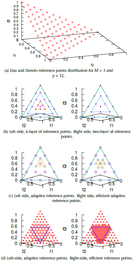
This task generates new reference points based on the adaptive and efficient adaptive reference points studied before, which are plotted in Figure 1d at the end of the IDTLZ1 optimization process (the left-side corresponds to adaptive reference points and the right-side to efficient adaptive reference points). One of the NSGA-III termination criteria is to have all reference points associated with each population member (
 = 1), thus indicating a well-distributed Pareto front. Notwithstanding, sometimes that is impossible because the amount of reference points is higher than the population size, and some of them have niche counts
= 0. They are relocated next to
crowded
reference points, and their capacity to capture a well-widespread Pareto front depends on the scaling factor λ and the settled down condition.
= 1), thus indicating a well-distributed Pareto front. Notwithstanding, sometimes that is impossible because the amount of reference points is higher than the population size, and some of them have niche counts
= 0. They are relocated next to
crowded
reference points, and their capacity to capture a well-widespread Pareto front depends on the scaling factor λ and the settled down condition.
Delete adaptive or efficient adaptive reference points
This task deletes existing reference points. It is required to associate the added reference points to the population and update the niche value
 (do not forget that

 = N for P
t+1
). The deletion function is computationally more expensive than the adding one. In this case, before deleting useless reference points, we need to repeat the association and niching procedures and steady-state new reference points insertion routines.
= N for P
t+1
). The deletion function is computationally more expensive than the adding one. In this case, before deleting useless reference points, we need to repeat the association and niching procedures and steady-state new reference points insertion routines.
The subsections below depict the constraint handling and the complexity discussion of EF1-NSGA-III algorithms.
Constraint Handling
We extended the constraint domination principle adopted in the NSGA-II algorithm for EF1-NSGA-III, A-EF1-NSGA-III, and A2-EF1-NSGA-III. It is handled automatically by the initialization process, where all population members satisfy the bounds. Also, the creation of offspring solutions must be within lower and upper bounds. The evaluation of each individual considers inequality constraints, which are configured in the problem definition function at the beginning of the simulation. When the non-dominated sorting procedure starts, all individuals within the combined population Rt = Pt U Qt are categorized as feasible and infeasible. x (1) is constraint-dominate x (2) if one of the following conditions is true. First, if x (1) is feasible and x (2) is infeasible. Second, if x (1) and x (2) are infeasible and x (1) has the smaller constraint violation. Third, if x(1) and x(2) are feasible and x (1) dominates x (2) with the usual domination principle.
There are four cases for the non-domination sort function in the tournament procedure to select individuals for the crossover function:
First, all solutions are infeasible; solutions are sorted by minimum violation values and copied to the next generation.
Second, the number of feasible individuals is lower than the population size; all feasible individuals are copied to the next generation.
Third, the number of infeasible individuals equals twice the population size; the unconstrained non-domination sorting procedure is followed.
Finally, the number of feasible individuals is higher or equal to the population size; the unconstrained non-domination sorting procedure is carried out with feasible individuals.
Complexity discussion
The NSGA-III and EF1-NSGA-III have a similar complexity because the EF1-NSGA-III inherits some of the NSGA-III procedures. The niche complexity requires O(N) computations, and the rest is bounded by the maximum between O(N 2 logM-2 N) and O(MN 2). However, if M > N2 logM-2 N, then he generation-wise complexity of the EF1-NSGA-III is O(MN2). The A-EF1-NSGA-II and A2-EF1-NSGA-III have a higher complexity, thus requiring more computations for each generation. In those cases, the complexity of the niche function is 2 * O(N).
Performance evaluation
In this section, we provide the performance results of EF1-NSGA-III, A-EF1-NSGA-III, and A2-EF1-NSGA-III to solve the DTLZ test (Deb, Thiele, and Laumanns, 2005) and real (water and car-side impact) problems handling constraints on three to ten objective functions. The employed hardware is a 3rd generation Intel core i7-3700x4 with 8 GBs of RAM, and the utilized software in Ubuntu 16.04, kernel 4.13.0-45-generic, and GCC version 5.4.0. We ran all the simulations using 20 realizations with the same random seeds for each problem.
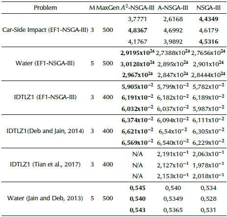
Additionally, we took the population and the number of reference points for each DTLZ test problem reported in Table I of the work by Deb and Jain (2014) and in Table 1 of this work. For tuning purposes, we used the NSGA-III parameters employed by authors. They are shown in Table II of Deb and Jain (2014), as well as here in Table 2.
Table 1 Reference points and population sizes used for EF1-NSGA-III, A-EF1-NSGA-III, and A2-EF1-NSGA-III algorithms. Nobj is the number of objective functions, and Boundary ndiv is the number of divisions of the boundary plane built with reference points. Within ndiv is the number of division of the inside plane built with reference points, and Popsize is the population size.
| Nobj | Boundary ndiv | Inside ndiv | H | Popsize |
|---|---|---|---|---|
| 3 | 12 | 0 | 91 | 92 |
| 5 | 6 | 0 | 210 | 212 |
| 8 | 3 | 2 | 156 | 156 |
| 10 | 3 | 2 | 275 | 276 |
Source: Authors
Table 2 Parameter values used in EF1-NSGA-III, A-EF1-NSGA-III, and A2-EF1-NSGA-III algorithms.
| Parameters | A/A2/EF1-NSGA-III |
|---|---|
| Simulated binary crossover probability p c | 1 |
| Polynomial mutation probability p m | 1/n |
| Distribution index for crossover η c | 30 |
| Distribution index for mutation η m | 20 |
Source: Authors
Traditionally, the ZDT (Zitzler, Deb, and Thiele, 2000), DTLZ (Deb et al., 2005), WFG (Huband, Hingston, Barone, and While, 2006), and LZ/UF (Li and Zhang, 2009)(Zhang and Li, 2007) test suites are commonly-used benchmark multi-objective test problems. They are employed to validate MOEAs and MaOEAs under some difficulties, such as objective scalability, complicated Pareto sets, bias, disconnection, or degeneracy (Li et al., 2018). There are even more tests and real problems to evaluate evolutionary algorithms (Surjanovic and Bingham, 2013). However, we concentrated our effort to benchmark DTLZ test problems with different versions of the NSGA-III. Along with the proposed algorithms, we compared our results with those reported by authors and some publicly available open-source versions in terms of Inverted Generational Distance (IGD) and HiperVolume (HV) performance metrics (Chiang, 2014; Tian et al., 2017; Bi and Wang, 2017; Blank and Deb, 2020).
Normalized DTLZ1-4 Test Problems
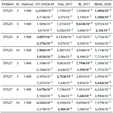
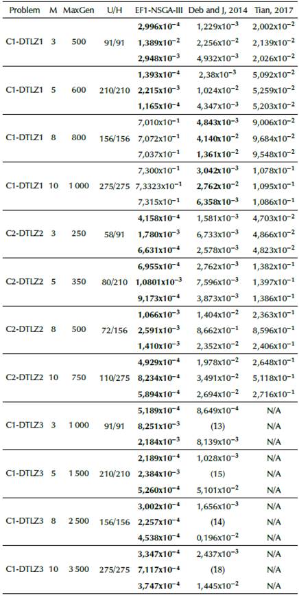
The original NSGA-III implementation (Deb and Jain, 2014; Jain and Deb, 2014), and others found in references of this work (Ariza, 2019; Chiang, 2014; Tian et al., 2017; Blank and Deb, 2020) find well-distributed solutions when solving MaOPs. We noticed that there is a small difference between them regarding the IGD performance metric on three-objective to ten-objective normalized DTLZ1-4 test problems, as summarized in Table 3. It shows that the EF1-NSGA-III outperforms most scenarios, followed by the proposals by Deb and Jain (2014), Blank and Deb (2020), Chiang (2014), and Tian et al. (2017). Nevertheless, it has poor performance when solving normalized eight-objective DTLZ1 test problems and above.
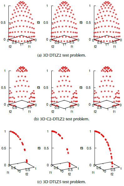
We visualized some three-objective problems solved with EF1-NSGA-III, A-EF1-NSGA-III, and A2-EF1-NSGA-III in Figure 2. They are DTLZ2 (Figure 2a), C2-DTLZ2 (Figure 2b), DTLZ5 (Figure 2c), DTLZ7 (Figure 2d), DTLZ1 (Figure 2e), DTLZ4 (Figure 2f), IDTLZ1 (Figure 2g), and Car-Side Impact (Figure 2h) problems, respectively. At first glance, The EF1-NSGA-III seems to achieve well-distributed and well-spread solutions for those problems. Also, the A2-EF1-NSGA-III performs better than the A-EF1-NSGA-III, and the latter is better than the EF1-NSGA-III for some DTLZ test problems with difficulties, for instance, in normalized DTLZ5, DTLZ7, and IDTLZ1 test problems.
Source: Authors
Figure 2. From left to right: Using the EF1-NSGA-III, EF1-A-NSGA-III and EF1A2-NSGA-III to solve three dimensional problems.
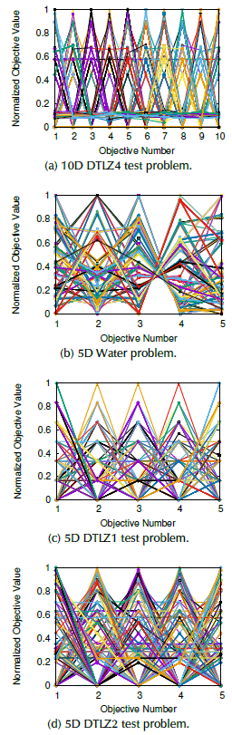
High dimensional problems are depicted in Figure 3 as well. In this case, we employed parallel coordinates plots to visualize the solutions for ten-objective DTLZ4 (Figure 3a), five-objective Water (Figure 3b), five-objective DTLZ1 (Figure 3c), and five-objective DTLZ2 (Figure 3d) problems, respectively.
Normalized DTLZ5 and DTLZ7 Test Problems
DTLZ5 and DTLZ7 test problems have irregular Pareto fronts that reveal the diversity maintenance of reference point adaption.
The DTLZ5 is a degenerate test problem whose Pareto Front lies on a dimension curve independent of the number of objectives. On the contrary, the DTLZ7 problem examines the algorithm's ability to sustain sub-population in different Pareto-optimal regions. Figures 2c and 2d depict the Pareto fronts of three-objective DTLZ5 and DTLZ7 problems. Other algorithms, such as Adaw (Li and Yao, 2020), have a consistently better distribution of solutions when solving both problems mentioned before. We observed that the EF1-NSGA-II is slightly better than other proposals in terms of the IGD metric, as shown in Table 4.
DTLZ1-5 and DTLZ7 Statistical benchmark
We made a statistical benchmark between EF1-NSGA-III and PYNSGA-III (Pymoo NSGA-III algorithm) in terms of IGD and HyperVolume (HV) performance metrics for DTLZ1-5 and DTLZ7 problems. Their statistical boxplots are shown in Figures 4 and 5 for three-objective and five-objective DTLZ problems running 20 realizations with the same random seeds. First, from an IGD perspective, we see in Figures 4a, 4b, 4c, 4d, 4e, and 4f, that the EF1-NSGA-III performs better than the PYNSGA-III and provides lower IGD values and dispersion. Notwithstanding, Figures 4g, 4i, 4j, 4k, 4l, and 4h depict a different scenario, where the PYNSGA-III performs better than the EF1-NSGA-III.
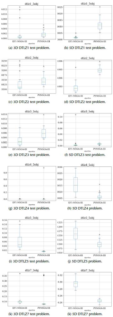
Then, when we analyzed the boxplots of Figure 5 related to the HV performance metric, we notice the same behavior obtained concerning the IGD performance metric. In this scenario, high HV values mean a better performance of convergence and distribution of solutions. That validation helps us be confident of the performance of the EF1-NSGA-III with respect to the PYNSGA-III. For example, Figures 5a, 5b, 5c, 5d, 5e, and 5f, accomplish a better performance in terms of HV for the EF1-NSGA-III rather than the PYNSGA-III. Hovewer, the PYNSGA-III performs better than the EF1-NSGA-III for DTLZ4, DTLZ5 and DTLZ7, as seen in Figures 5g, 5h, 5i, 5j, 5k and 5l.
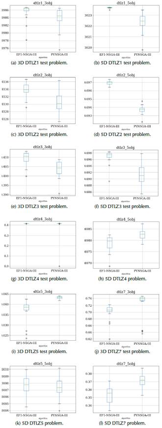
Exceptionally, the EF1-NSGA-III strives to solve the DTLZ4 test problem for five objectives and above, and those drawbacks are represented with a significant data dispersion, as shown in Figures 4h and 5h. This kind of convergence difficulty occurs for some seeds, so the idea is to increase the number of realizations to reduce this effect.
Inverted-DTLZI Test Problem
The inverted-DTLZ1 problem is an unconstrained test problem that modifies the DTLZ1 problem. The DTLZ1 transformation requires f i (x) = 0,5(1 + g(x)) - f i (x), for i = 1,...,M objectives. We can see that the A2-EF1-NSGA-III distributes the population better than the A-EF1-NSGA-III and the EF1-NSGA-III. The Hyper-volume values are shown in Table 5 and visually confirmed in Figure 2g. We employed the same algorithm from reference (Blank and Deb, 2020) to evaluate the HV. It takes the obtained Pareto front from EF1-NSGA-III and PYNSGA-III and a reference point. We used the point [0,6, 0,6, 0,6] for the three-objective IDTLZ1 problem, the point [39,4,12,5] for the Car-side impact problem, and the point [75000,1400, 2900000, 6700000, 26000] for the water problem to obtain HV values. Sometimes, for instance, the Car-side impact problem solved with the EF1-NSGA-III has better HV values than the A2-EF1-NSGA-III and the A-EF1-NSGA-III. It remains as future work where the number of realizations should be increased.
Table 5 Best, Worst and Median Hyper-volume values obtained for A2-NSGA-III, A-NSGA-III and NSGA-III
Source: Authors
Normalized constrained DTLZ test problems
We considered three cases of constrained DTLZ test problems. The first is the C1-DTLZ1 problem that uses the constraint c(x) = 1 -
 ≥ 0. The second is the C1-DTLZ3 problem that employs the constraint c(x) =
 ≥ 0, where r = {9,12,5,12,5,15,15} is the radius of the hyper-sphere for M = {3,5,8,10,15}. Finally, the C2-DTLZ2 problem that utilizes the constraint c(x) =
 where r = 0,4 for M = 3 and 0,5 otherwise.
Table 6 shows a consistently better performance of the EF1-NSGA-III in terms of IGD for the studied constrained problem, except for C1-DTLZ1 on eight-objective to ten-objective problems, where the EF1-NSGA-III gets stuck. The approximated Pareto-front of C2-DTLZ2 is depicted in Figure 2b that shows a good distribution of solutions.
Table 6 Best, Worst and Median IGD values obtained for NSGA-III. Constrained DTLZ problems
Source: Authors
Car-Side Impact and Water Problems
The Car-Side Impact problem optimizes the frontal structure of the vehicle for crash-worthiness. It minimizes the weight, the pubic force experienced by a passenger, and the V-Pillar's average velocity to resist the impact load. Its mathematical formulation can be consulted in Jain and Deb (2014). We can see, in Figure 2h, that the A2-EF1-NSGA-III has a better distribution of solutions compared to the A-EF1-NSGA-III and EF1-NSGA-III. Nevertheless, in Table 5, we notice that the EF1-NSGA-III achieves better HV values than the A2-EF1-NSGA-III or the A-EF1-NSGA-III. It is necessary to use statistical analysis with more realizations to better understand the distribution of solutions.
Conversely, as shown in Table 5 and Figure 3b, the Water problem has better performance when it is solved with the A2-EF1-NSGA-III, A-EF1-NSGA-III, and the EF1-NSGA-III, which is expected. This problem has five objective functions, three design variables, and seven constraints. Its mathematical formulation is found in the work by (Jain and Deb, 2014).
Variation of convergence metrics
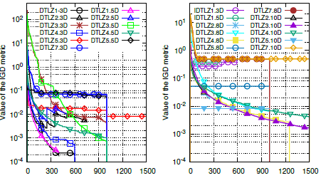
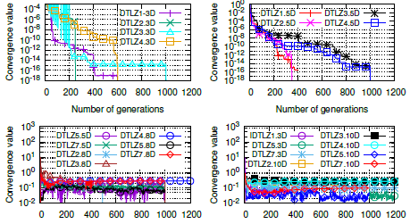
We used IGD and Y values in each generation to visualize the convergence. IGD convergence is depicted in Figure 6 and the Y convergence in Figure 7. The IGD convergence plot is divided into two cases. The first (Figure 6 on the left side) contains better IGD decreasing performance for DTLZ1, DTLZ3, DTLZ4, DTLZ5, and DTLZ7 problems. However, the DTLZ1 is the fastest. In contrast, the second (Figure 6, on the right side) shows bad decreasing IGD performance for IDTLZ1, DTLZ5, and DTLZ7 problems. They will not achieve good performance even though we increase the number of generations. High dimensional DTLZ3 and DTLZ4 problems probably will achieve a good IGD value, but they require significantly more generations. We also divided the Y convergence plot in two cases. The first (Figure 7, top side) for low dimensional cases, and the second, for high dimensional cases (Figure 7, bottom side). We noticed that this metric is representative for problems up to eight objectives. We also saw that the DTLZ1, DTLZ2, DTLZ3, and DTLZ4 problems exhibit better Y convergence, but DTLZ3 and DTLZ4 problems require more generations to accomplish similar Y values. Finally, high dimensional test problems did not provide good Y values, as shown in Figure 7, bottom part.
Conclusions
We successfully extended the NSGA-II algorithm from the KanGAL's Code to the EF1-NSGA-III, the A-EF1-NSGA-III, and the A 2 -EF1-NSGA-III. These algorithms have been applied to solve constrained and unconstrained Many-objective optimization problems (up to ten-objective problems). Our proposals have shown their niche in finding a set of well-converged and well-diversified solutions repeatedly over multiple runs. They are susceptible to be employed as a reference for a comparative evaluation of new evolutionary algorithms because they yield consistently better results than those reported in references (Deb and Jain, 2014; Jain and Deb, 2014; Bi and Wang, 2017; Tian et al., 2017; Chiang, 2014; Blank and Deb, 2020).

