Introduction
In recent years, the ability to generate and store data has far outpaced the capability to analyze and exploit it (Rydning 2018). According to Gantza and Reisel (2012), just 3% of global data are currently tagged and ready for manipulation, and only 0,5% of this is used for analysis, at least in 2012.
Therefore, the interest in analyzing and extracting useful information to understand phenomena or for decision-making has brought the attention of practitioners and the research community. The increasing production of temporal data, especially time series, has motivated the analysis for extracting valuable knowledge through knowledge discovery in databases (KDD) processes and data mining (DM) techniques (Sun, Yang, Liu, Chen, Rao, and Bai 2019, Boulle, Dallas, Nakatsukasa, and Samaddar 2020).
Time series are an important class of temporal data objects, and they can be easily obtained from scientific research (Fu 2011) and other domains such as medicine, engineering, earth and planetary sciences, physics and astronomy, mathematics, environmental sciences, biochemistry, genetic and molecular biology, agricultural and biological sciences, among others.
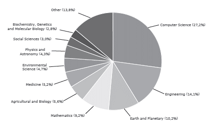
Figure 1 shows a scientific document analysis by subject areas where time series have been used, especially in classification tasks during the last seven years, obtained from the Elsevier-Scopus database, where 7 973 articles were considered.
Source: Authors
Figure 1 Analysis of the time-series usage that has been reported in scientific documents in the last seven years.
Time series T = (t 1 ,...,t n ) ∈ℛ is the result of the observation of the underlying procedure in which a set of values is collected through measurements made into uniformly spaced time-instants. Therefore, a time series can be defined as an ordered sequence of n real-valued variables (Esling and Agon 2012, Jastrzebska 2019).
A wide variety of DM techniques has been proposed and applied to dealing diverse tasks in domains where time series can be involved (Gong, Chen, Yuan, and Yao2019, Jastrzebska 2019, Ali, Alqahtani, Jones, and Xie 2019).
However, classical DM techniques often perform poorly in the presence of time-series data, because most of them treat time-series as unrelated data, thus resulting in inaccurate or inconsistent models (Rashid and Hossain 2012).
To overcome the disadvantages of traditional DM techniques with time series, a set of techniques has been proposed which are part of Temporal Data Mining (TDM). TDM has a huge array of techniques for tackling tasks such as query by content, clustering, classification, segmentation, and others (Yang 2017).
When time series data are involved in the data mining process, the quality of the mined data can depend on two important issues: the first is the choice of the appropriate algorithm for a given task, while the second is the proper hyper-parameter selection that may produce a relatively good performance.
Both issues are known as algorithm selection (AS), and model selection (MS), and these are often solved separately. Nevertheless, there are some proposals which have addressed both AS and MS at the same time under the issue known as full model selection (FMS) (Escalante, Montes, and Sucar 2009).
Therefore, FMS consists of finding an appropriate set of methods and their hyperparameter optimization for multitasking. This combination can be represented as a kind of pipeline, characterized by avoiding the dependency on user knowledge (Hutter, Kotthoff, and Vanschoren 2019).
Multiple approaches have been proposed to find automated pipelines according to the hyperparameter optimization process (Yu and Zhu 2020). These approaches can be categorized into three main classes: a) approaches based on exhaustive traditional search (Bergstraand Bengio 2012), b) approaches based on Bayesian optimization (Shahriari, Swersky, Wang, Adams, and de Freitas 2016), and c) approaches based on metaheuristics (Hutter et al. 2019).
The first class of these approaches can be impractical and costly because the search focuses on exhaustive exploration defined for a particular block of the pipeline. In contrast to exhaustive approaches, Bayesian approaches keep track of past evaluation results, which they use to find better model settings than random search in fewer iterations. The major drawback of Bayesian optimization approaches is that inference time grows cubically in the number of observations.
Metaheuristics represent a flexible option that has been increasingly used to build optimized pipelines. Population-based metaheuristics such as evolutionary or swarm intelligence algorithms have been adopted to propose an automatic framework that finds streamlined pipelines (Sun, Pfahringer, and Mayo 2013, Olson, Urbanowicz, Andrews, Lavender, Kidd, and Moore 2016, de Sá, Pinto, Oliveira, and Pappa 2017).
Most of the population-based metaheuristic approaches have focused on building pipelines for databases in which the temporary factor is not considered. Therefore, approaches dealing with FMS while involving the building of time series pipelines are scarce.
Single-point search, a part of metaheuristics, has been used for search optimized structures or hyperparameter selection (Aly, Guadagni, and Dugan 2019). Local search is an example of a single-point search that has turned out to be a practical option to solve complex problems despite being the most straightforward.
In this paper, an architecture is proposed for finding an optimized pipeline for time series databases in which the FMS problem is related. It is empirically studied from two points of view: the first, from a population-based approach, where μ-DE is used as a search engine; and the second, from a single-point search, where a local search is adopted.
The main objectives of this work are to empirically study the proposed architecture, varying the search engine and solution encoding; and to offer an alternative that automatically assists the selection of an optimized pipeline for time series database tasks, i.e., to solve the FMS problem for time series.
Related works
From the literature review, it is essential to note that FMS is not a new trend. Since the 90s, solutions have emerged to deal with the issue of selecting an algorithm from a portfolio of options in order to carry out a single task (Rice 1976).
Subsequently, the need arises to incorporate more tasks into said selection (multi-task) and deal with hyperparameter optimization, resulting in machine learning pipelines (Hutter et al. 2019).
Nowadays, learning pipelines are developed to be truly usable by a non-expert. Against this background, a need for automated machine learning (AutoML, a recently coined term) systems can be used to handle various tasks and solve the FMS problem, a challenging and time-consuming process.
Grid search, random search, Bayesian optimization, and metaheuristics are four conventional approaches to building AutoML systems for diverse applications (Bergstra and Bengio 2012). Grid search and random search are traditional hyperparameter optimization methods that could prove impractical to explore high-dimensional spaces at a high computational cost.
Bayesian optimization has been effective in this realm and has even outperformed manual hyperparameter tuning by expert practitioners. Auto-WEKA (Hall et al. 2009), mlr (Bischl et al. 2016) and auto-SKLearn (Pedregosa et al. 2011) are approaches based on Bayesian optimization, and their prime objective is to find the best combination between complete learning pipelines and their respective parameters.
Both approaches follow a hierarchical method that first chooses a particular algorithm and, only after this step, optimizes its parameters. Thus, algorithms may be left out which, with the right hyperparameters, could generate better results than the selected ones.
On the other hand, metaheuristics, especially evolutionary and swarm intelligence algorithms, have gained a particular interest in the research community by allowing the construction of machine learning pipelines that can be complex and extensive.
In the rest of this section, a set of metaheuristics-based approaches for AutoML are described.
Metaheuristics-based approaches
In 2009, Escalante etal. (2009) proposed a machine learning pipeline that included selecting a preprocessing algorithm, a feature selection algorithm, a classifier and, all their hyper-parameters. Their approach used a modified Particle Swarm Optimization (PSO) to deal with the limited configuration space and was called PSMS system. Although the authors found that they could apply their method to different datasets without domain knowledge, most of the datasets used had unrelated attributes. In order to avoid overfitting, the authors proposed using k-cross-validation, and then the approach was extended with a custom assembling strategy that combined the best solutions from multiple generations (Escalante, Montes, and Sucar 2010).
Later, Sun et al. extended the idea of PSMS and proposed the unification of the PSO algorithm and the Genetic Algorithm (GA) (2013). This approach was called GPS (which stands for GA-PSO-FMS). A GA were was used to optimize the pipeline structure, while the PSO for the hyperparameter optimization of each pipeline. The pipeline proposed by the authors included selecting from a pool of methods such as data sampling, data cleansing, feature transformation, feature selection, and classification. The datasets used for evaluating GPS were characterized by a high number of instances, thus causing an increase in the computational cost during the loss function evaluation. Therefore, the authors proposed the use of an internal binary tree structure to speed up the GPS system.
Another interesting line of research is the application of multi-objective evolutionary algorithms. One of these approaches is the Multi-objective Support Vector Machine Model Selection (MOSVMMS) (Rosales-Pérez, Escalante, Gonzalez, Reyes-Garcia, and Coello-Coello 2013), where the search is guided by a Non-dominated Sorted Genetic Algorithm-II (NSGA-II).
The authors built a pipeline formed by feature selection, pre-processing, and classification tasks focused only in the SVM classifier. The models were evaluated under bias and variance trade-off as prime objective functions. This approach was only tested on thirteen binary classification problems. Two extensions of this approach were reported, the first called Multi-Objective Model Type Selection (MOMTS), where a multi-objective evolutionary algorithm based on decomposition (MOEA/D) was used instead of the NSGA-II (Rosales-Pérez, Gonzalez, Coello-Coello, Escalante, and Reyes-Garcia 2014). MOMTS focused only on selecting classification models without other involved tasks. However, the authors explored the idea of measuring complexity models through the Vapnik-Chervonenkis dimension, which could have a high computational cost as the dimension of the datasets grows.
For that reason, the second extension proposed by Rosales-Pérez, Gonzalez, Coello, Escalante, and Reyes-Garcia was the Surrogate Assisted Multi-Objective Model Selection (SAMOMS) (2015), in which a pipeline structure is considered, (preprocessing, feature selection, and classification). They proposed a surrogate assistant to speed up the fitness evaluation.
The Tree-Based Pipeline Optimization Tool (TPOT) is an open-source software package for configuring pipelines in a more flexible manner (Olson et al. 2016). TPOT uses a genetic programming algorithm for optimizing structures and hyperparameters. The main operator included in TPOT has supervised classification, feature preprocessing operators, and feature selection operators, all ofthem taken from scikit-learn. The main drawback of TPOT is considering unconstrained search, where resources can be spent on generating and evaluating invalid solutions.
So far, these approaches do not present evidence of the treatment of time-series databases. Most of them use a fixed pipeline length in sequential steps. TPOT is, to date, the approach that stands out for optimizing the design of pipes. Early efforts for an approach that suggests automated pipelines for time series can be found a previous work proposed by Pérez-Castro, Acosta-Mesa, Mezura-Montes, and Cruz-Ramírez (2015). The authors proposed using a micro version of differential evolution to solve the FMS problem, and they suggested optimized pipelines. In that work, smoothing, time series representation, and classification through the k-nearest neighbor algorithm are only considered. This work is an extension of the work mentioned above.
FMS problem in time-series databases
The FMS term, conceived by Escalante et al. (2009), consists of selecting a combination of suitable methods to obtain a learning pipeline for a particular database with a low generalization error.
In this paper, the FMS problem in time series databases is tackled as a single-objective optimization problem, defined by Equation (1), based on the definition made by Díaz-Pacheco, Gonzalez-Bernal, Reyes-García, and Escalante-Balderas (2018), which consists of searching for suitable pipeline composed by a smoothing s* λ Є S, a time series representation r* λ Є R, a numerosity reduction e* λ Є E, and classification method c* λ Є C with their related hyper-parameter setting A from the corresponding domain space ∧.
For each pipeline, a loss function ℒ is estimated over a labeled time-series database
 , where for
 , which denotes an ordered sequence of n real-valued variables (univariate time series), and yi e Y for the corresponding label value.
In order to build pipelines with a low generalization error, database D is divided into k disjoint partitions (D (i) t and D (i) v for i = 1,2,...,k).
Where, S is the set of available smoothing methods; R is the set of available time series representation methods; E is the set of available numerosity reduction methods; C is the set of available classifiers; λ is a vector of hyperparameters; D t is a training data partition; D v is a validation partition; ℒ is a loss function computed on the validation set; and argmin returns the lowest values estimated by the loss function.
Methodology overview
Materials
Benchmark databases
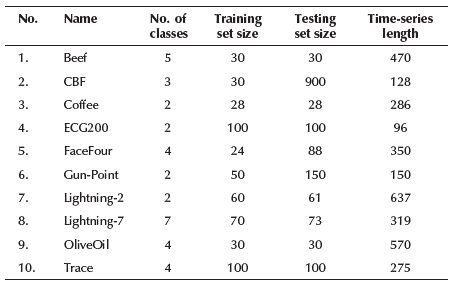
In this article, a part of the well-known collection of univariate time series databases is used (Keogh et al. 2011). The essential characteristics of those databases are summarized in Table 1.
A brief description of each database is presented below:
Beef: This database consists of five classes of beef spectrograms acquired from raw samples, cooked using two different cooking regimes. Each beef class represents a differing degree of contamination with offal (Al-Jowder, Kemsley, and Wilson 2002).
CBF: Cylinder-Bell-Funnel is a simulated database where each class is standard normal noise plus an offset term that differs for each category (Saito 2000).
Coffee: The coffee database consists of two spectrograms class that distinguish between Robusta and Arabica coffee beans (Bagnall, Davis, Hills, and Lines 2012).
ECG200: The electrocardiogram (ECG) database contains the measurements recorded by one electrode during one heartbeat. The two classes correspond to a normal heartbeat and a myocardial infarction, respectively (Olszewski 2001).
FaceFour: This database was built from face profile images. Each time series was obtained by converting a local (outer) angle at every point x of the face profile contour, starting from the head profile's neck area (Keogh et al. 2011).
Gun-Point: This database was obtained from motions with hands involving one female actor and one male actor. Two classes were identified: Gun-Draw (actors point the gun at a target for approximately one second) and Gun-Point (actors point with their index fingers to a goal for about one second). Each time series corresponds to the centroid of the actor's right hands in the x-axis (Ratanamahatana and Keogh 2005).
Lightning-2 and Lightning-7: The FORTE satellite detects transient electromagnetic events associated with lightning using a suite of optical and radio-frequency (RF) instruments. Data is collected with a sample rate of 50 MHz for 800 microseconds that are transformed into spectrograms, which are collapsed in frequency to produce a power density time series, with 3 181 samples in each time series. These are then smoothed to produce time series of length 637 and 319 (Eads et al. 2002).
OliveOil: This is another example of the food spectro-graphs used in chemometrics to classify food types. Each class of this database corresponds to virgin olive oils originating from four European producing countries.
Trace: It is a synthetic database created by Davide Roverso and designed to simulate instrumentation failures in a nuclear power plant. All instances are linearly interpolated to have the same length of 275 data point (Roverso 2000).
It can be seen that most databases describe real phenomena. A behavior analysis of time-series databases was carried out. This analysis consisted of observing three characteristics: a) class separation (CS), b) noise level (NL), and c) the similarity between the training and testing sets (SBS). The mean, median, and average of these per class for each database were computed and plotted from raw databases. From the visualization, the three characteristics of the above-listed were ranked. CS 1 means non-separable, and a value of 3 means easily separable. NL can take values between 1-5, where 1 means low noise and five high noise. SBM was measured in a range of 1 to 3, where 1 represents low similarity, and 3 means high similarity. The results of this analysis are summarized in Table 2.
Table 2 Characteristics of visual analysis in time-series databases
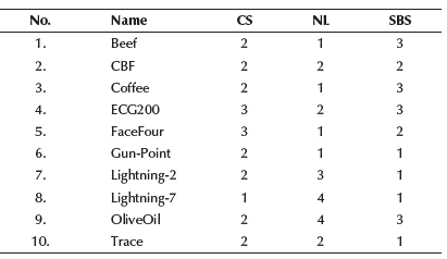
Note: Acronyms: CS (Class Separation); NL (Noise Level); SBS (similarity between the training and testing sets)
Source: Authors
It is important to note that the data was not pre-processed for the experimental stage.
Pipeline tasks: available methods
In this work, four main tasks are considered to build a learning pipeline for time series which involves solving the FMS problem.
Smoothing: It is usually used to soften out the irregular roughness to see a clearer signal. This task does not provide a model, but it can be a promising first step in describing various series components (Giron-Sierra 2018). It is common to use the term filter to describe the smoothing procedure. Moving Average (Baijal, Singh, Rani, and Agarwal 2016), the Savitzky-Golay filter (Savitzky and Golay 1964), and Local Regression (with and without weights) are considered with related hyper-parameters (Cleveland and Loader 1996).
Time-series representation: This task consists of transforming the time series to another domain to reduce dimensionality, followed by an indexing mechanism. Piecewise Aggregate Approximation (PAA) (Keogh, Chakrabarti, Pazzani, and Mehrotra 2001), Symbolic Aggregate approximation (SAX) (Lin, Keogh, Wei, and Lonardi 2007) and Principal Component Analysis (PCA) are available methods (Page, Lischeid, Epting, and Huggenberger 2012).
Numerosity reduction: It is a procedure used to reduce data volume by using suitable forms of data representation. The Monte Carlo 1 (MC1) and INSIGHT approaches were included (Garcia, Derrac, Cano, and Herrera 2012, Buza, Nanopoulos, and Schmidt-Thieme 2011).
Clasification: It is a machine learning supervised task that consists of identifying the category to which a new observation belongs, based on a training set of data containing examples whose category membership is known. Some classifiers were considered, such as k-nearest neighbors, Naive Bayes, among others (Bishop 2006).
Table 3 shows a summary of the available methods for each pipeline tasks and their related hyperparameters.
Table 3 Description of available methods for each pipeline task and the description of their hyperparameters (values in square brackets indicate lower and upper limits)
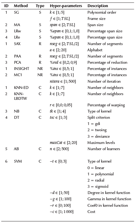
Note: Acronyms: S (Smoothing); R (Representation); NR (Numerosity Reduction); C (Classification); TLS (Time-series length); SG (Savitzky-Golay Filter); MA (Moving Average); LRw (Local Regression-lowess); LRe (Local Regression-loess); SAX(Aggregate approximation); PAA (Piecewise Aggregate Approximation); PCA (Principal Component Analysis); INSIGHT (Instance Selection based on Graph-coverage and Hubness for Time-series); MC1 (Monte Carlo 1); KNN-ED (K-Nearest Neighbor-Euclidean Distance); KNN-LBDTW (K-Nearest Neighbor-Lower Bounding Dynamic Time Warping); NB (Naive Bayes); DT (Decision Tree); AB (AdaBoost); SVM (Support Vector Machine)
Source: Authors
Encoding pipeline solutions
A candidate solution for the learning pipeline for time-series databases is represented as a vector in this work. Each vector can be formed by continuous values, binary values, or mixed values (continuous and discrete values).
Continuous encoding: Each potential solution is encoded as a continuous vector which is formed as in Equation (2).
Where depicts each position within a particular vector; and X j,s Є [1;4], X j,r Є [1;3], X j,e Є [1;2], and x j , c Є [1;6] represent the ID of the selected smoothing, time-series representation, numerosity reduction, and classification available methods, respectively.
h j,1 ...,ns, h j,1,…, nr, h j,1,…,ne , and h j , 1,…,nc encode the set of hyperparameters related to the overall available methods, where ns, nr, ne, and nc represent the number of hyperparameters per type of task into the learning pipeline that has different limits. Each position can take random continuous values according to Equation (3), which determines a value between the lower and upper bounds of each hyperparameter, described in Table 3.
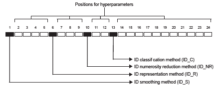
In Equation (3), lb i is a lower bound, ubi an upper bound, and rand represents a random value between 0 and 1. Figure 3 shows an example of the structure of a continuous vector solution. Black boxes represent the positions that encode the selected method according to the task in the learning pipeline (smoothing, time-series representation, numerosity reduction, and classification), and the white boxes encode their related hyperparameters. For continuous encoding, vectors of 24 dimensions are considered to represent a learning pipeline, which is equivalent to a candidate solution of FMS problem for time-series databases.
Source: Authors
Figure 2 Graphical representation of a solution encoding used in contentious or mixed encoding.
Mixed encoding: Mixed encoding consists of a vector of 24 dimensions, as shown in Figure 2. However, for this option, both continuous and discrete values are permitted.
Continuous values are generated by Equation (3), according to the limits of each position. In contrast, discrete values are generated by randi(), the function of MATLAB language that returns integer values drawn from a discrete uniform distribution, where limits are also respected.
Binary encoding: Binary encoding consists of a vector formed by binary values (0 or 1). These values can be grouped into binary strings that represent continuous or discrete values.
The length of a particular binary string depends on the boundary of values to be expressed. Binary string length lj is computed with Equation (4), where int expresses a integer value, log 2 is the log base 2, ub the upper boundary, lb the lower boundary, and precision is a constant that means the number of decimal places to encode.
Then, the overall binary vector length bvl to encode a potential pipeline solution is the concatenation of each binary string. Equation (5) states how it is computed, where D is the amount of continuous or discrete values that can be encoded as binary strings, and l j is the maximum length of these binary strings.
If a mixed vector structure is considered containing 24 values that represent a potential pipeline solution, which respects the boundaries of the values presented in Table 3, then vector with a length of 169 positions is required. It can be seen in Figure 3 that the first three binary values correspond to a binary string representing integer values between 1 and 4 that are the number of available smoothing methods. The next binary strings encode the rest of the values.
A decoding process is needed to compute the quality of each binary encode solution. Decoding is performed for each binary string xs of complete binary vector according to Equation (6), where lbj is the lower boundary used for this binary string, ub j is the upper boundary used for this binary string, xint is the result of traditional binary to decimal conversion, and l j is the binary string length performed obtained from (4)
Fitness function
The Cross Validation Error Rate (CVER) is used as the fitness function f x to evaluate the quality of a learning pipeline under a particular time-series database. Equation (7) describes fx, where a represents the portion of instances in the time-series database that was incorrectly classified, and b is the total number of instances in such database. k depicts the number of stratified subsamples (folds) chosen randomly but with roughly equal size in the cross validation method that is adopted to avoid over-fitting.
Methods: search engines
Micro Differential Evolution (μ-DE)
Population-based metaheuristics such as evolutionary algorithms have a reduced population version that has proven to be efficient for solving large scale optimization problems (Olguín-Carbajal et al. 2019, Salehinejad, Rahnamayan, and Tizhoosh 2017). The reduced population versions usually are denoted with the prefix u Besides the small population, μ algorithms are characterized by a restart mechanism to avoid stagnation.
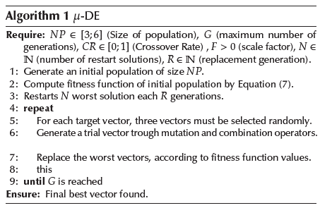
The μ-DE cycle and conventional operations, based on the scaled difference between two vectors of a population set, remain the same as in the classical DE. Usually, the population size in μ -DE can take a value between four and six vectors (Viveros Jiménez, Mezura Montes, and Gelbukh 2012, Caraffini, Neri, and Poikolainen 2013). Regarding the restart mechanism, μ -DE requires randomly replacing the N worst vectors each R generations. In this paper, the u-DE proposed by Parsopoulos (2009) is used as a population-based metaheuristic.
Algorithm 1 summarizes the main steps of the adopted u-DE. Step six shows the mutation and combination process, for that, different variants such as rand/1/bin, rand/1/exp, best/1/bin, and best/1/exp are used in the experimentation.
This results in four versions to solve FMS problem, called P-DEMS1 (Population-Differential Evolution Model Selection 1, using rand/1/bin), P-DEMS2 (Population-Differential Evolution Model Selection 2, using rand/1/exp), P-DEMS3 (Population-Differential Evolution Model Selection 3, using best/1/bin), and P-DEMS4 (Population-Differential Evolution Model Selection 4, using best/1/exp).
Local search (LS)
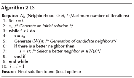
LS, a single-point optimization metaheuristic, is considered to be the oldest and most straightforward method (Talbi 2009). However, it has recently been used to train complex structures of neural networks and examine their hyperparam-eters for successful image classification (Aly et al. 2019). The LS algorithm used in this paper is briefly described in Algorithm 2.
For each iteration of the LS, a single solution s is replaced by a neighbor as long as the objective function is improved. Otherwise, the original solution is preserved. The search stops when all candidate neighbors are worse than the current solution, meaning that a local optimum is reached.
Step five (Algorithm 2) corresponds to the operator that generates the N neighbors of a slightly varied solution, according to the type of solution encoding. The neighbors are generated based on nvar Є [1; D] modifications that equivalent to the selected random positions. For example, Figure 4a shows a binary vector where nvar = 3. Thus, 3 positions are switched (0 instead 1 or vice-versa).

Source: Authors
Figure 4 Examples of neighbors generated by LS. (a) Using a binary encode. (b) Using mixed encode.
On the other hand, when mixed encoding is used, the nvar selected values are replaced with new values that are within boundaries of their corresponding variables (Figure 4b).
Two versions of LS are adopted as search engines: S-LSMS1 (Single-Local Search Model Selection, where binary encoding is used) and S-LSMS2 (Single-Local Search Model Selection, where mixed encoding is used).
Methodology architecture
In this section, the general architecture adopted for evaluating both population-based and single-point search approaches for solving the FMS problem to find a suitable learning pipeline for time-series databases is described.
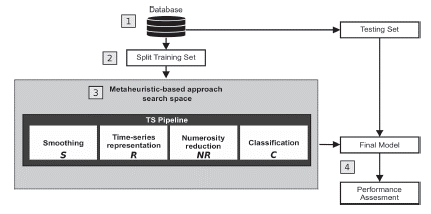
The architecture can be summarized into four main steps (Figure 5).
A training time-series database is considered as input data.
The training database is split into k stratified subsets (each subset contains approximately the same percentage of samples of each target class as the complete set) that are available during the search process.
This step consists of the search process guided by the metaheuristics, either the population-based or single-point versions. Regarding population-based options (based on Algorithm 1), these generate random solutions according to continuous encoding. The overall population is evaluated thought the fitness function (Equation 6) under the stratified subsets generated in the second step. The solutions evolve throughout an established number of iterations, and, in the end, the best solution is obtained. Regarding single-point search (based on Algorithm 2), a unique solution is generated (binary or mixed encoding) which improves throughout the iterations. In the end, the best solution is also obtained.
The final best solution found in the search process is evaluated with the test database.
Experiments and results
This section presents a set of experiments where the PM (population-based metaheuristics) versions and SM (single-point-based metaheuristics) are used as the search engines to solve the FMS problem and find a suitable pipeline for time-series databases.
The experimentation is presented in five subsections: (1) a comparison ofthefinal statistical results of each metaheuristic, (2) a convergence plot analysis, (3) a diversity analysis of the PM versions, (4) an analysis of the final obtained models, and (5) a frequency analysis of the methods' usage. Each metaheuristic was evaluated in the ten time-series databases described in Table 1. Considering the high computation time required by the approaches, five independent runs for each metaheuristic were carried out. The termination condition was 3 000 evaluations. The configuration used by each involved metaheuristics is described in Table 4, based on (Viveros-Jiménez et al. 2012, Escalante et al. 2009).
Table 4 Experimental settings for each metaheuristic approach

Note: Acronyms: PM (Population-based Metaheuristic); SM (Single-point-based Metaheuristics); f-DE (micro Differential Evolution); LS (Local Search); I (Iterations); NP (Population Size); CR (Crossover Rate); F (Scaled Factor); N (Number of restart solutions); R (Replacement generation); Nk (Number of neighbors)
Source: Authors
Final Statistical Results
Table 5 shows the final numerical results of CVER obtained by the six metaheuristics versions. The reported values correspond to the average of five trials evaluated in the testing set of each database.
Table 5 Comparison of averaging performance among the six metaheuristics for each database

Note: Acronyms: P-DEMS1 (Population-Differential Evolution Model Selection 1 with rand/1/bin); P-DEMS2 (Population-Differential Evolution Model Selection 2 with rand/1/exp); P-DEMS3 (Population-Differential Evolution Model Selection 3 with best/1/bin), and P-DEMS4 (Population-Differential Evolution Model Selection 4 with best/1/exp); S-LSMS1 (Single-Local Search Model Selection with binary encoding); S-LSMS2 (Single-Local Search Model Selection with mixed encoding). Values to the right of ± represent the standard deviation, the values in parentheses represent the ranks computed by the Friedman test, and values in parentheses to the left mean the lowest values found or the best ranking.
Source: Authors
Due to the fact that the samples have a non-normal distribution, and multiple comparisons are needed, the non-parametric Friedman test was used (García, Fernández, Luengo, and Herrera 2010). The related samples are the performances of the metaheuristics measured across the same data sets. The Friedman tests evaluates the following null hypothesis: all methods obtain similar results with non-significant differences.
In the Friedman test, numerical results are converted to ranks. Thus, it ranks the metaheuristics for each problem separately. The best performing metaheuristic should have rank 1, the second best, rank 2, etc., as shown in Table 5. When there are ties, average ranks are computed. With six compared metaheuristics and ten databases, the p-value computed by the Friedman test was 0,183, which means that the null hypothesis is accepted. Thus, there are no significant differences found among the compared metaheuristics.
However, according to the average rank shown in Table 5, the S-LSMS1 (SM with binary representation) was the highest rank in most of the databases. It was followed by the P-DEMS1 (PM based on μ-DE, where the base vector is randomly chosen, and a binomial crossover is used).
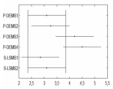
To enhance statistical validation, the Tukey post-hoc test based on the Friedman results was applied by using the best and median values obtained over the five runs for each metaheuristic over the whole databases. Figures 6 and 7 show the results of this test, where the x-axis exhibits the confidence interval of mean ranks (given by the Friedman test) and the y-axis shows the name of each metaheuristic compared. Using the best and median values, the test yielded a p-value = 0,005 and a p-value = 0,250, respectively. In the case of Figure 6, there was a significant difference between S-LSMS1 and P-DEMS4.
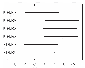
Source: Authors
Figure 7 Tukey post-hoc test using the median values over the whole set of databases.
Meanwhile, in Figure 7, there are no significant differences between the metaheuristics. Finally, a pairwise comparison was conducted to determine which of the metaheuristics exhibit a different performance against a selected control metaheuristic, namely S-MSLS1 because it was the best ranked.
The non-parametric 95% confidence Wilcoxon rank sum test was applied to the numerical results of the six metaheuristics for each database. Table 4 shows the numerical results of the pairwise comparison. The metaheuristics are sorted according to the average rank provided by the Friedman test.
The results in Table 6 show that the S-LSMS1 technique was able to provide the most competitive results among the compared metaheuristics. S-LSMS1 outperformed P-DEMS1 in two (out often) databases Lightning-7 and Trace, while P-DEMS1 outperformed S-LSMS1 in Coffee and GunPoint. S-LSMS1 outperformed P-DEMS2 in four databases (Beef, ECG200, Lightning-7, and Trace), while P-DEMS2 outperformed S-LSMS1 in just the Coffee database.
Table 6 Comparison between the control metaheuristic S-LSMS1 and the rest of metaheuristics

Note: Acronyms: P-DEMS1 (Population-Differential Evolution Model Selection 1 with rand/1/bin); P-DEMS2 (Population-Differential Evolution Model Selection 2 with rand/1/exp); P-DEMS3 (Population-Differential Evolution Model Selection 3 with best/1/bin), and P-DEMS4 (Population-Differential Evolution Model Selection 4 with best/1/exp); S-LSMS1 (Single-Local Search Model Selection with binary encoding); S-LSMS2 (Single-Local Search Model Selection with mixed encoding). (-) means that there was a significant difference favoring the control metaheuristic. (+) implies that there was a significant difference favoring the compared metaheuristic. (=) means that no significant difference was observed between the compared metaheuristics. Values in parentheses to the left mean the best values found.
Source: Authors
S-LSMS1 outperformed S-LSMS2 in Beef and Lightning-7, and was beaten in the Coffee database. S-LSMS1 outperformed P-DEMS4 in four databases (Beef, ECG200, Lightning-7, and Trace) and was outperformed in just one (Coffee). In summary, S-LSMS1 was able to obtain the best numerical values at least in eight often databases (Beef, CBF, ECG200, Face-Four, Lightning-2, Lightning-7, OliveOil, and Trace). Finally, P-DEMS3 was outperformed by S-LSMS1 in three databases (ECG200, Lightning-7, and Trace) and outperformed in just one (Coffee).
Analysis of convergence plots
To further understand the behavior of each compared meta-heuristic, the convergence plots of a set of representative databases are analyzed.
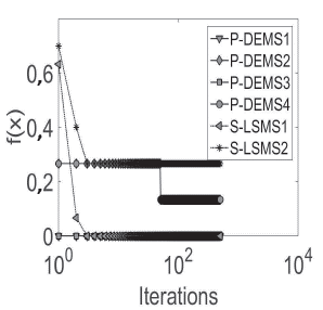
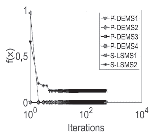
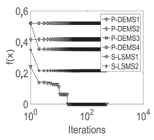
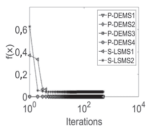
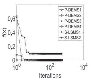
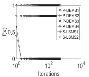
The average of five independent runs for each database is plotted. From Figures 8 to 13, convergence plots for Beef, CBF, Gun Point, Lightning-2, OliveOil, and Trace are shown. The x-axis represents the number of performing iterations for each metaheuristic, and the y-axis represents the fitness function value obtained for each iteration.
The x-axis was plotted in the logarithmic scale for a better display of the results. The results suggest that, in the case of the ,u-DE, to obtain a fast and competitive solution, the best option is P-DEMS1, which uses a random base vector and binomial crossover.
However, in cases such as in the Trace database, PDEMS1 was trapped in local optima. Regarding SMs, S-LSMS2 (mixed representation) achieves fast convergence with respect to S-LSM1 (binary representation), but the first is usually caught in local optima, e.g., Beef, CBF, Lightning-2, or OliveOil, while S-LSM2 finds better values.
Finally, an important finding is that P-DEMS1 had a faster fitness improvement in early iterations, i.e., before 100 iterations in most databases. However, S-LSMS1 was capable of finding competitive final results at the end of the search process.
Diversity analysis of population-based metaheuristics
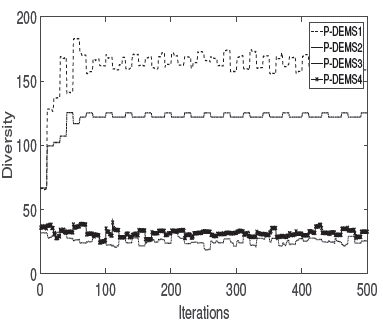
According to Yang, Li, Cai, and Guan (2015), the population diversity has a strong influence on the performance of evolutionary algorithms. Therefore, a brief analysis of population diversity in PM versions is presented. The diversity measure is based on the distance between vectors in the variable space. For each iteration, a centroid is computed in the current population.
Then, the Euclidean distance is calculated between each vector of the population and the centroid vector. With the aim of measuring the individuals' dispersion, the standard deviation over the whole distances at the current population is computed. The diversity measure was computed for each PM over the five independent runs per each database.
Figure 14 shows the averaging diversity measure of each PM over the ten databases. A high diversity in P-DEMS 1 is observed against the other f-DE versions. It can be said that the use of a random base vector instead of the best one, as well as the binomial instead of the exponential crossover, favors a better diversity maintenance.
Analysis of final pipeline-models
Table 7 shows the best pipelines suggested by each compared approach for each database. The third column details the pipeline models. Despite the fact that differences were observed in the solution models, there are interesting similarities.
Table 7 Best final pipelines obtained by each approach for all databases
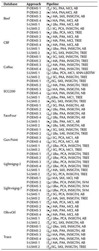
Note: Acronyms: S (Smoothing); R (Representation); NR (Numerosity Reduction); C (Classification); TLS (Time-series length); SG (Savitzky-Golay Filter); MA (Moving Average); LRw (Local Regression-lowess); LRe (Local Regression-loess); SAX(Aggregate approximation); PAA (Piecewise Aggregate Approximation); PCA (Principal Component Analysis); INSIGHT (Instance Selection based on Graph-coverage and Hubness for Time-series); MC1 (Monte Carlo 1); KNN-ED (K-Nearest Neighbor-Euclidean Distance); KNN-LBDTW (K-Nearest Neighbor-Lower Bounding Dynamic Time Warping); NB (Naive Bayes); DT (Decision Tree); AB (AdaBoost); SVM (Support Vector Machine); P-DEMS1 (Population-Differential Evolution Model Selection 1 with rand/1/bin); P-DEMS2 (Population-Differential Evolution Model Selection 2 with rand/1/exp); P-DEMS3 (Population-Differential Evolution Model Selection 3 with best/1/bin), and P-DEMS4 (Population-Differential Evolution Model Selection 4 with best/1/exp); S-LSMS1 (Single-Local Search Model Selection with binary encoding); S-LSMS2 (Single-Local Search Model Selection with mixed encoding). Symbols in parentheses mean the spent runtime during training and the subscripts represent the performance of the pipeline in terms of classification error. (|) means high runtime > 933 minutes, (•) means medium runtime > 272 and < 873 minutes, (J.) means low runtime < 272 minutes. Subscripts next to symbols: g means good, r means regular, and b means bad performance.
Source: Authors
Regarding the smoothing task, Moving Average was the most preferred. PAA was the most commonly used and suggested method for time series representation, while INSIGHT was the most popular numerosity reduction technique.
As for the classification task, the decision tree and the Ad-aBoost (with decision trees as the weak learners) appeared as the most suitable. From the resulting final models, it can be seen that there were some evaluated databases with different models with similar performance values.
Databases such as Beef, Gun-Point, and Lightning-7 were detected as possible multimodal problems. They reported more diversification in the selected methods and their related hyperparameters.
Runtime varies considerably due to the different features of the temporal databases and the selected methods for carrying out a specific sub-task. Overall, P-DEMS3 reported the lowest runtime computational cost, while S-LSMS1 was the most expensive approach.
However, S-LSMS1 reported the best performance during training and competitive results in the testing phase. Figure 15 shows a graphical example of the suggested pipeline that was applied to the CBF database. It can be seen that the average behavior of the original CBF database remains after the processing originated by the applied pipeline. A significant dimensionality reduction was observed.
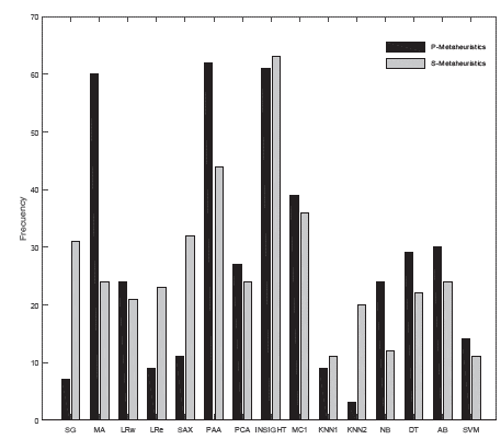
Note: Acronyms: P-Metaheuristics (Population-based Metaheuristics); S-Metaheuristics (Single point search Metaheuristics); SG (Savitzky-Golay Filter); MA (Moving Average); LRw (Local Regression-lowess); LRe (Local Regression-loess); SAX(Aggregate approXimation); PAA (Piecewise Aggregate Approximation); PCA (Principal Component Analysis); INSIGHT (Instance Selection based on Graph-coverage and Hubness for Time-series); MC1 (Monte Carlo 1); KNN1 (K-Nearest Neighbor-Euclidean Distance); KNN2 (K-Nearest Neighbor-Lower Bounding Dynamic Time Warping); NB (Naive Bayes); DT (Decision Tree); AB (AdaBoost); SVM (Support Vector Machine). Source: Authors
Figure 15 Frequency analysis of included into pipeline task by metaheuristics.
Frequency analysis of considered method by metaheuristics
In order to enhance the analysis of the preferred solutions, a selection frequency analysis of the methods considered by the approaches for the FMS problem in time-series databases was made. Figure 16 shows the average frequency, for each recognized method, computed from five trials over all databases for each metaheuristic.
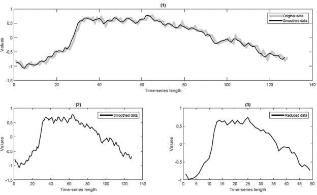
Note: (1) The average behavior of the original testing database is plotted that is compared to the average smoothed testing test. (2) The averaged smoothed testing database is plotted before the time-series representation process. (3) The averaged smoothed testing database is plotted after the time-series representation and numerosity reduction processes were applied. Source: Authors
Figure 16 Example of pipeline-model applied to CBF database. Model: S:MA{span = 67}, R:PAA{nseg=21}. R:MC1{%ins=0.81403,nitera=400}, C:AB{n = 436}.
The frequency results for population-baed meteheuristics were based on 601 200 evaluated pipeline-models, while single-point search metaheuristics were based on 300 600 models. Regarding the smoothing options, Moving Average method, was the most solicited by population-based meteheuristics, while the Savitzky-Golay filter was the most preferred by single-point search metaheuristics.
For time-series representation, the PAA method was the most preferred for both population-based and single-based metaheuristics. INSIGHT was the most selected numerosity reduction method. Regarding the classifiers, it can be confirmed that Adaboost was the most suitable classifier, while KNN1 was the less preferred.
Conclusions and future work
In this paper, a comparison study between two metaheuristic approaches to deal with FMS and pipelines building for time-series databases was presented. The first approach was based on the micro-version of a differential evolution algorithm, named as ¡u-DEMS in this work, from which four variants were tested based on rand/1/bin (P-DEMS1), rand/1/exp (P-DEMS2), best/1/bin (P-DEMS3), and best/1/exp (PDEMS4).
The second approach focused on evaluating local search behavior S-LSMS, the most straightforward single-point search metaheuristics. Two versions were assessed, one of them with binary encoding and the second one with mixed encoding.
Six complete pipeline-model search options were evaluated, out of which four are P-DEMS variants and two are S-LSMS variants. Each of the variants was evaluated in ten different time-series databases.
The set of experiments was divided into five parts: the statistical analysis of the numerical results, the analysis of the convergence graphs, a diversity analysis focused only on the population variants, the analysis of the final pipeline models, and the study of the selection frequency of the methods involved. From these experiments, some important conclusions and findings are listed below:
Statistical analysis suggests that S-LSMS1 (binary encoding version) is the best option when working with time-series databases that have high dimensionality, are noisy, and whose number of classes is higher than two, such as Lightning-2, Lightning-7, and OliveOil. S-LSMS1 has the advantage of being simple in its structure, and only requires two parameters to be set. However, it has the disadvantage of having a high computational cost.
On the other hand, if the database is dichotomous, the noise is moderate, and its dimensionality length is below an approximate value of 350. Therefore, population-based metaheuristics P-DEMS1, which uses rand/1/bin, turns out to be the best option. Besides, it achieved competitive results around the first 100 iterations.
Regarding the exploration capacity, it was observed that the population-based metaheuristic P-DEMS1 with therand/1/bin variant provides a better diversity of pipeline models.
With respect to the final pipeline-models, it can be seen that, for most of the databases, a complete model was found which contained the most straightforward methods for the tasks of smoothing, dimensionality reduction, and number reduction. These methods are Moving Average, PAA, and INSIGHT, respectively. On the side of the classification task, AdaBoost was the most common method.
An important finding was discovering different complete pipeline model configurations with similar performance for the same database. Therefore, some temporary databases can be seen as a multi modal problem.
As part of future work, a complexity measure could be considered as a fitness function to then tackle the FMS problem as a multi-objective problem. Additionally, a mechanism to build more flexible pipelines where the length and order can incorporated, in addition to searching for a way to fairly compare it against other state-of-the-art approaches.


