


 English (pdf)
 Article in xml format
 Article references
 Send this article by e-mail
 Cited by SciELO
  Cited by Google
  Similars in
SciELO
Similars in
SciELO  Similars in Google
 Permalink
Introduction
Fractured media refers to lowpermeability matrix rocks that may acquire moderate to good permeability thanks to fractures (Singhal and Gupta, 2010). There, underground projects for groundwater supply, waste disposal, or infrastructures are built up (Evans et al., 2001; Singhal and Gupta, 2010), thus affecting the surrounding surface water sources and groundwater bodies. Some of the reported effects of tunnels are groundwater inflows during and after their construction (Celico et al., 2005; Perrochet and Dematteis, 2007), groundwater and surface water level drawdown, (Molinero et al., 2002; Maréchal and Etcheverry, 2003; Vincenzi et al., 2009; Font-Capóet al., 2011), the triggering of preferential flow paths (Evans et al., 2001), and rock deformations and instabilities (Preisig etal., 2014; Shen et al., 2014; Loew et al., 2015; Valenzuela et al., 2015).
Different modeling approaches have been implemented to assess the impact of underground projects both in the transient and steady state. In the steady state analysis, long term effects are studied, whereas in the transient state, the effects during the construction process are analyzed until a new steady state condition is reached (Celico et al., 2005). Some analytical formulations based on the equivalent porous media (EPM) approach have been developed for steady state conditions and homogeneous materials (Goodman et al., 1965; Heuer, 1995; Karlsrud, 2001; El Tani, 2003), and some have been extended to the transient-state. Perrochet (2005) evaluates the transient drilling speed-dependent discharge rates using a convolution integral, and extensions to the heterogeneous media have been proposed by Perrochet and Dematteis (2007) and Maréchal et al. (2014). Previous approaches do not consider the effect of the excavation-induced drawdown leading to over/underestimated groundwater inflows. For this reason, some authors have proposed analytical or semianalytical approaches to predict the height of lowered water level under the steady (Su et al., 2017) and the transient states (Liu et al., 2017), thus providing a better prediction of tunnel inflows.
Since most groundwater inflows are recorded in fault zones (Attanayake and Waterman, 2006; Perrochet and Dematteis, 2007; Yang et al., 2009; UNAL, 2010; Moon and Fernandez, 2010; Zarei et al., 2011; Loew et al., 2015), fractures have been represented within heterogeneous media as more permeable areas with EPM approaches (Perrochet and Dematteis, 2007; Maréchal et al., 2014; Preisig, 2013). This conceptualization has been extended to numerical modeling in order to predict groundwater inflow into tunnels (Maréchal et al., 1999; Hu and Chen, 2008; Yang et al., 2009; Butscher etal., 2011; Chiu and Chia, 2012; Butscher, 2012; Xia et al., 2018; Golian et al., 2018; Nikvar Hassani et al., 2018).
Even though the EPM approach allows the use of the above-mentioned analyses while the characterization of individual fractures, the complexity of the fractured media could be better represented by discrete fracture networks (DFN), where hydraulic behavior is controlled by their geometry (i.e., aperture, length, density, and orientation distributions) (Adler et al., 2012).
The inclusion of individual fractures or fracture networks in numerical modeling demands higher computational efforts to solve the problem. Nevertheless, some authors have included fractures on their analyses while accounting for the water management in tunnels (Molinero et al., 2002; Lee et al., 2006; Hawkins et al., 2011; Hokr et al., 2012, 2016; Farhadian etal., 2016). Recently, Wang and Cai (2020) proposed a DFN-DEM multi-scale approach for modeling excavation responses in jointed rock masses for settlement purposes. However, the use of synthetic DFNs to estimate groundwater inflows into tunnels or underground works under a transient state has not been reported. In this study, we propose a numerical model to analyze the temporal evolution of groundwater inflows (hydrograph) during the construction of underground works in a fractured massif with a low permeability matrix. The novelty of this work is that its conceptual model is based on a hybrid model with a DFN embedded on a low-permeability, continuous porous media. The generation of the synthetic DFN was carried out using the probabilistic functions of (i) frequency, (ii) length, (iii) aperture, and (iv) dip of the fractures. The groundwater flow model is bounded with a time-varying atmospheric pressure, which is activated according to a typical drilling speed of 2 m/d (Perrochet and Dematteis, 2007).
To show the capabilities of the proposed model, two types of simulation were performed. The first one is a hypothetical case with a randomly generated fracture network where the numerical model is tested. The second one consists of an embedded synthetic discrete fracture network (DFN) that is generated based on outcrop field data with information from surveys on La Línea massif in the Colombian Andes. The former only gives us information on the numerical performance of the groundwater model, whereas the second model is compared to the groundwater inflows recorded during the drilling of the La Línea tunnel (Colombia).
Methodology
The release of energy above the plastic limit fractures the rock Escobar, 2017, thus generating faulted planes that provide preferential flow paths through the massif rock (Leung and Zimmerman, 2012), which enhances the permeability of the media. Fractures are characterized by their length, surface roughness, aperture, fracture dead-end, and intersections (Adler et al., 2012). These geological measurements are used to estimate hydraulic parameters (Liu et al., 2016) by using frequency distributions such as the power law, lognormal, or exponential functions.
Fracture lengths have shown power-law distributions to have the greatest physical significance (Bonnet et al., 2001) and ubiquitously describe scaling properties (Davy et al., 2010). However, in nature, the frequency of fracture lengths displays log-normal (Equation (1)) or exponential distributions (Equation (2)) as result of the truncation effect induced by the sampling size, which limits the lower or upper boundary (Bonnet et al., 2001).
where μ is the log-mean, σ is the log-standard-deviation, λ is a parameter of the exponential distribution, l is the fracture length, and n(l) is the frequency distribution of fracture lengths.
Meanwhile, aperture distribution cannot be obtained easily from field measurements, which are uncertain because stresses change dramatically at depth (Liu et al., 2016), and the weathering affects fracture appearance at outcrops. DFNs are realistic mappings of fracture geometries based on field observations via a stochastic representation of properties (Somogyvári et al., 2017) such as fractures number, length, aperture, and dip. Their statistical parameters are the inputs for several codes developed to generate and analyze DFNs, such as ADFNE (Fadakar Alghalandis, 2017), DFN WORKS (Hyman et al., 2015), FracMan (Golder Associates Inc., 2018), and MoFrac (Mirarco, 2018). Nevertheless, these codes do not allow to simulate the advance in tunnel drilling processes, as it could be done using codes such as HydroGosSphere HGS (Aquanty Inc., 2013).
HGS is a 3D, fully integrated surface and subsurface flow simulator that is widely used in the analysis of groundwater issues (Aquanty Inc., 2013). It includes a Random Fracture Generator (RFG) that creates networks with random locations, lengths, and apertures by using any of the available probability distribution functions (PDF): exponential function for the aperture, exponential and lognormal functions for the fracture length, and a double-peaked Gaussian for the orientation. In this research, HGS and RFG were used to generate a synthetic DFN embedded on a very low permeability porous rock matrix.
In the following sections, we present the assumptions of the model components (mesh, DFN generation, definition of hydraulic parameters) and describe the initial and boundary conditions for the numerical simulations. All these components are described for both hypothetical and synthetic cases.
Mesh generation
The accuracy of groundwater models is affected by numerical errors or instabilities that occur in all computational simulations due to aspects such as grid spacing (Woods et al., 2003; Anderson et al., 2015). To ensure numerical stability in the modeling process, multiple preliminary simulations were performed, varying the number of fractures, block size, and grid spacing. Different block sizes were tested according to the width of the fault zones in the La Línea tunnel, which varies approximately from 20 m to 400 m, as well as to the total length of tunnel (8 600 m). Block size and grid spacing were identified as the most important aspects to guarantee a successful run, the availability of computational requirements, and a moderate simulation time. As result, a synthetic block of 400 m in length and height, 200 m in depth (which could be a representative volume for the La Gata, Alaska, or Cristalina fault zones in the La Línea massif), and mesh spacing varying from 1 to 80 m were chosen. In the middle of the block, the mesh was refined to simulate a tunnel with a radius of 2,5 m. That position was chosen to avoid boundary disturbances and aimed for symmetrical conditions. Mesh spacing limits the shortest fractures, while the model size limits the longest fractures. Usingthis scheme, each groundwater flow simulation took about 60 minutes using an Intel Xeon (@ 3.30GHz) and 32 GB RAM.
Synthetic DFN generation
RFG was used to create a DFN based on the statistical parameters of length, aperture, orientation, and number of fracture distributions. Fractures were randomly distributed in the porous media using a seed that can be changed to allow the generation of a infinite number of different DFN with the same PDF for each fracture parameter. The resulting three-dimensional model is made of orthogonal blocks, where fractures are superposed as 2D elements to the sides of the 3D blocks, so that the fracture nodes coincide with those of the porous rock. The grid has to be thin enough to allow the creation of the fracture network. Nevertheless, extremely thin grids increase the number of elements and computation times.
A hundred DFN realizations for different configurations or settings were performed by varying density (expressed as the number of fractures generated) and fracture length parameter distributions (Equations (1) and (2)), while length distribution, grid, model dimensions, and hydraulic parameters were kept constant. However, some realizations could not be completed because of numerical instabilities.
DFN hydraulic properties
The hydraulic properties were used as indicators of DFN connectivity. Here, we considered the hydraulic conductivity of each fracture, Kf, the permeability of the fracture network (KDFN), the volumetric fracture density (P 32 ), and the equivalent permeability (Kepm) associated to the DFN mean flow (Qdfn).
HGS estimates Kf by following the cubic law as
 , where g[L/T2] is gravity acceleration, Wf [L], is the aperture, and v[M/(L-T)] is the kinematic viscosity (Aquanty Inc., 2013). Thus, the permeability of the fracture network, KDFN, was evaluated as thegeometric mean of the Kf (de Dreuzy, 2001a). The volumetric fracture density, P
32
, or the persistence of the fractures area (2D) per unit volume (3D), is expressed as
, where g[L/T2] is gravity acceleration, Wf [L], is the aperture, and v[M/(L-T)] is the kinematic viscosity (Aquanty Inc., 2013). Thus, the permeability of the fracture network, KDFN, was evaluated as thegeometric mean of the Kf (de Dreuzy, 2001a). The volumetric fracture density, P
32
, or the persistence of the fractures area (2D) per unit volume (3D), is expressed as
 , where V is the volume of model, A
f
is the area of the fracture f, If is the length, and b the width of the model.
, where V is the volume of model, A
f
is the area of the fracture f, If is the length, and b the width of the model.
As each setting had as many hydrographs as completed simulations, an equivalent DFN hydrograph (Qdfn) was calculated: Q
dfn
= Σ QDFNi/N, where N is the number of completed i synthetic generations. Then, an equivalent porous media permeability (KEPM) for each setting was calibrated based on 200 realizations in a homogeneous media configuration (EPM), where K was varied; specific storage, Ss, remained constant as the assigned value of the matrix domain in the DFN approach. In this way, a set of 200 EPM hydrographs Qepm were obtained, and Q
dfn
was fitted to the set of Qepm using the Nash-Sutcliffe coefficient (NSE
 ; NSE values close to unity indicate good model performance) as the metric to select the KEPM.
Hydraulic properties of the matrix
The matrix was considered as a very low permeable medium with a hydraulic conductivity (K) of 1 x 10⁻⁴ m/d, specific storage (Ss) equal to 5 x 10⁻⁴, and porosity (/]) equal to 4 x 10⁻³ (Singhal and Gupta, 2010).
Initial and boundary and conditions
An initial condition of head equal to topography is assigned to the entire domain. No flow conditions are assigned to the bottom and lateral faces of the cubic domain, considering the following assumptions specifically for the La Línea massif : i) preferential radial flow toward the tunnel (Preisig, 2013); ii) there are no significant regional flows, as the tunnel is located in the upper watershed; and iii) very low permeabilities of the crystalline rocks (IRENA, 2010; UNAL, 2015). These assumptions may be rejected due to possible connections with larger faults. However, it is an open issue when working with fractures and the consequent truncation effect due to the scale of the observation window.
A nodal flux of 1 x 10⁻¹⁰ m3/d is assigned to the top face as an arbitrary recharge condition, in order to avoid a constant drawdown. The tunnel is simulated with a mobile boundary condition along the x-axis, in the middle of the y - z plane. The advance of the tunnel drilling is simulated by assigning an atmospheric pressure at an excavation rate of 2 m/d (typical value for tunnel excavation rates (Perrochet and Dematteis, 2007; IRENA, 2007)). Tunnel excavation is completed in 200 days, and the recession flow is observed until 1 000 days.
Test cases
Two example cases were investigated using synthetic DFN in the analysis of groundwater inflows into a tunnel. The first case was a hypothetical block to test the performance of the numerical modeling. The second case was based on outcrop field data from the La Línea massif and the recorded groundwater inflows of the Alaska fault zone during the drilling of the La Línea tunnel.
Hypothetical case
In this case, the behavior of the hydrographs was analyzed by varying the fracture length, aperture, and density distributions. Six settings were built (each one with 100 realizations). The fracture length frequency was assumed tofollowa log-normal distribution with μ= -4,5 m and σ = 3,4 m, whereas the exponential distribution was used for the fracture apertures. The fracture density or number of fractures was randomly assigned. Settings S1, S3, and S4 have the same density but their exponent λ varies from 8 000 to 10 000, while, in settings S2, S5, and S6 the exponent λ is kept constant (it is equal to 9 000). The parameters for each setting are displayed in Table 1.
The Alaska fault zone
As an application example, and based on the results from the hypothetical case, the Alaska fault zone was analyzed using five different settings, where fracture density was varied, and fracture length followed the statistical distribution of the La Línea massif.
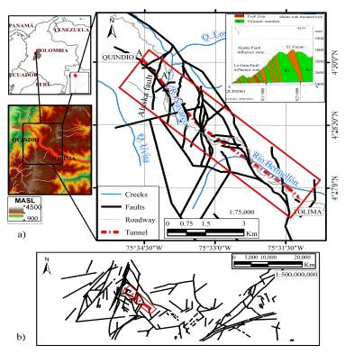
The Alaska fault is located in the La Línea massif and is crossed by the drilling of two tunnels (Figure 1). These tunnels belong to an important roadway project in the Colombian Andes.
Source: Authors
Figure 1 Geographical location of the La Lánea tunnel: a) Location of the Alaska fault and fractures at a local scale (10000 m); and b) fractures at a regional scale (50 000 m).
Their mean length is 8 600 m, the elevation at the East entrance is 2 434 m.a.s.l., 2 553 m.a.s.l. in the West, and the maximum depth is 800 m. The massif is formed by the Quebradagrande complex, the Cajamarca complex, and an andesithic porphyry. These geological formations are highly fractured and formed by igneous and methamorphic rocks with a complex structural geology (IRENA, 2007; UNAL, 2010). During the drilling process, important groundwater inflows were recorded, especially in faultzones (IRENA, 2007; UNAL, 2010). The Alaska fault zone is located in shales of the volcanic member of the Quebradagrande complex, Kv, as shown in Figure 1. The mean depth of the tunnel in the zone is 400 m.
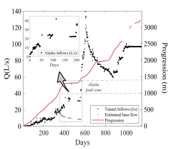
When a tunnel is being drilled, there is a flow peak as the drilling front disturbs the rock followed by the recession flow, which diminishes or disappears depending on the hydrogeological conditions. In this way, the total amount of water drained by a tunnel is the convolution of each individual hydrograph. In the La Línea tunnel, the accumulated groundwater inflows were measured daily at each entrance of the tunnel (IRENA, 2007). However, there is no information on the real infiltration rates in specific zones. Hence, based on the average of 100 numerical simulations using an EPM approach, the recession flow of the first 1 000 m of tunnel is obtained and then removed from the accumulated data. Figure 2 displays the inflows recorded at the western entrance and the progression in the drilling front (IRENA, 2007); the hydrograph of the infiltrated water in the Alaska fault zone (inner box in Figure 2) was built subtracting the aforementioned recession or base flow (gray line). There, the drilling process took about 200 days, and about 40 l/s were recorded.
Source: Authors
Figure 2 Daily groundwater inflows (black dots) and tunnel progression (red line); base flow (gray dots) was removed from accumulated hydrograph to obtain the Alaska inflows shown in the inner box (2007).
Fracture length distribution: The statistical parameters of the fracture lengths are obtained from structural maps at local and regional scale (10000 m and 65 000 m, respectively) (Figure 1), considering that just few and small outcrops (less than 30 m) are found as consequence of the dense vegetation in the area.
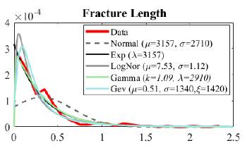
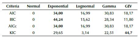
Finding the best statistical distribution governing a dataset is of critical importance when predicting the tendency of fracture attributes (Rizzo et al., 2017). The information criterion approach is implemented using the Akaike Information Criterion AIC (Akaike, 1974), the corrected AICc (Cavanaugh, 1997), the Bayesian Information Criteria BIC (Schwarz, 1978), and the KIC (Kashyap, 1982). Then, the estimation of the posterior model weight (for AIC and AlCc) or posterior model probability (for BIC and KIC) is implemented, as described in detail by Ye et al. (2008) and Siena et al. (2017). Fracture length was fitted to five probability density functions (normal, exponential, lognormal, gamma, and General Extreme Value-GEV) using the Maximum Likelihood Estimator approach. The four information criteria indicate the best fit for the exponential distribution with the lowest values. The same result is obtained by the posterior model weight or posterior model probability (showing the higher values) using the AIC, AlCc, and BIC (Table 2). However, the KIC posterior probability is better for the GEV distribution, as it discriminates the models on the quality of the model parameter estimates (Siena et al., 2017). Therefore, the exponential distribution is selected for the DFN generations of the Alaska fault zone with λ = 3,16 x 10³ m. The data fit is shown in Figure 3.
Source: Authors
Figure 3 Probability density functions for fracture length in Alaska fault zone in the La Línea tunnel.
Table 2 Posterior weights/model probability of the five analytical models evaluated for the model identification criterion
Source: Authors
An example of the synthetic DFN generated using the log-normal (hypothetical case) and the exponential distribution for the fracture length with the same number of fractures is shown in Figure 4.
Source: Authors
Figure 4 Example of the generated DFN: (a) hypothetical case and (b) application example for the Alaska fault zone.
Fracture aperture: Regarding the aperture information, it was not possible to obtain aperture measurements within the massif, or any information to estimate a real value. Mean aperture measurements on surface were 1,5 mm, the minimum was 0 mm, and the maximum was 32 mm (Hernandez and Kammer, 2016). These values are extremely high, as result of the weathering of the outcrops. They do not even allow running the model because of numerical convergence issues. However, preliminary tests showed that the default HGS aperture distribution approach worked fine. Consequently, the aperture generation range was kept between 25 pm and 3,2 x 102 μm, and λ equal to 9,0 x 10³ for the exponential distribution (Equation 2).
Results
Hypothetical case
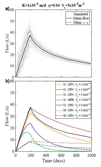
Figure 5a displays the hydrographs for each completed generation in S1, the estimated mean, and the standard deviation (σ). Peak groundwater inflows vary between 28 and 52 L/s, and the recession flows are less spread than those observed for early times. In the estimation of KEPM, it is important to consider that HGS changes the time step to optimize CPU requirements; when the simulated variable shows large variations, time steps are smaller. On the contrary, if no sensible variation is simulated, the time steps increase. After 200 days, when excavation is finished, and hydraulic heads do not vary significantly, the time step increases, and only ten values are generated in the remaining 800 days. For this reason, when the NASH coefficient is calculated, differences between Q EPM and Qdfn in the recession zone of the hydrograph are not so relevant, and the NASH coefficient values are close to one.
Source: Authors
Figure 5 Hydrographs of the simulated groundwater inflows for DFN generations: a) setting 1 (S1); b) mean flow obtained using the DFN and EPM approaches using different fracture densities (settings S1 and S6) and DFN approach for S1, showing the influence of Ss (m-1) in the simulated flows.
Table 3 contains K EPM , NASH, and K DFN for each setting. K EPM varies between 8 x 10⁻³ and 4 x 10⁻² m/d, while KDFN ranges from 5 x 10² to 6 x 10² m/d. The difference between both approaches (KEPM and KDFN) exceeds 5 orders of magnitude. Therefore, the values are not comparable, and the assumption of an equivalent permeability of the media, estimated as KDFN and proposed by de Dreuzy et al. (2001b), does not work in this study. It may be associated to the matrix of low permeability and P32 below 1 used in this research. Consequently, the effects of matrix permeability and fracture density should be taken into account for future modeling and analysis.
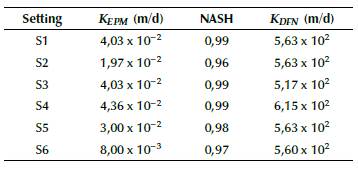
Figure 5b displays the calculated QDFN for different fracture densities in settings S1 and S6, and QEPM, showing how flow increases as the number of fractures does. The excavation phase shows a good fit between EPM and DFN (until 200 days). However, the tail of the hydrograph is overestimated by the EPM approach, which leads us to perform a sensitivity analysis of the Ss for S1, showing how the peak and the recession flow decrease as a function of Ss.
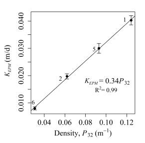
Based on the obtained results, DFN hydraulic parameters (introduced in the section named after them) were estimated and compared with previous studies (de Dreuzy et al., 2001b; Maillot et al., 2016) in order to validate the behavior of the generated DFN. Figure 6 displays the relationship between permeability and P32 for the settings where only the fracture density changes (S1, S2, S5, and S6). A linear relationship between the KEPM and the P32 is observed, as found by Maillot et al. (2016), but in a lower density range, considering that the estimated P32 for the analyzed configuration is below 1.
The Alaska fault zone
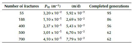
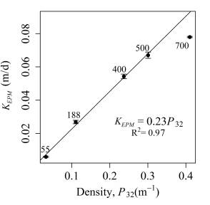
In this subsection, the results of a more complex fracture network (Figure 1) are presented. The statistical properties for the fracture lengths of the maps (Figure 2) were taken to configure the DFN generation, and the fracture density was varied from 55 to 700 fractures, as indicated in Table 4. As the density changes, connectivity does as well, and, consequently, Kepm (Table 4). However, in this application, the linear relationship observed in the synthetic example (Figure 6) and reported by Maillot et al. (2016) is not preserved for the most dense setting (700 fractures), as shown in Figure 7. It is probably a truncation effect caused by the lower number of numerically successful runs (55 of 100 simulations) caused by the difficulty to locate a higher number of fractures in the same domain size and mesh distribution.
Table 4 Density and K EPM for five settings with different number of fractures implemented for the Alaska fault zone
Source: Authors
Source: Authors
Figure 7 Relationship between permeability and fracture density P32 for the Alaska fault zone, displaying the 95% confidence interval bars of the K EPM (tags indicate the number of fractures in each setting).
Finally, by visual inspection, the synthetic DFN with about 400 fractures generates hydrographs that show a good agreement with the measured inflows in the first 100 days (Figure 8). Unfortunately, there are no records for 60 days, probably as a result of construction problems due to rock quality and the presence of water, which caused the drilling advance to be almost stopped. This would explain the decrease in the flows from 180 to 200 days, followed by a sudden increase as tunnel blasting was resumed. This kind of situation during construction activities is the greatest limitation in the acquisition of information for every geological unit, in addition to the complexity involved in the behavior of the recession flow.
Discussion
The accurate distribution of fractures in a rock massif is almost impossible to know. Synthetic DFN generations can be used as a tool to model the effects caused by tunnel drilling through fault zones, considering the daily advance in the perforation work.
Figures 6 and 7 show how geological media permeability is heavily dependent on DFN density, P32. However, for the application example of the Alaska fault zone, a perfectly linear relationship is not observed. This may be associated to a truncation effect in the fractures.
The behavior of high-density DFNs in a very low permeability matrix has important characteristics: groundwater must flow through fractures, so that the DFN has to be connected in order to contribute to groundwater circulation. In the porous the statistical parameters of the structural geology of a massif (i.e., fracture length and aperture measured in geological maps or outcrops), synthetic DFNs can reproduce groundwater inflows of the same order of magnitude than those measured in the Alaska fault zone in the La Línea tunnel, Colombia. This is an outstanding finding of this research, as the results were compared with real data, which has never been reported before. Unfortunately, there are no available measured data of the hydrograph at late times for this specific zone, so Ss estimation is an open issue. As input information of a fracture network is scarce, uncertainty is high. However, it can be established that fracture density, P 32 , is the parameter that most influences the estimated EPM permeability for the conditions of this study, which is in agreement with Maillot et al. (2016). The relationship between P 32 and equivalent permeability is heavily influenced by the fracture length distribution. Thus, a linear performance cannot be always supposed, probably because of the truncation effect caused by the size of the synthetic model.

