


 English (pdf)
 Article in xml format
 Article references
 Send this article by e-mail
 Cited by SciELO
  Cited by Google
  Similars in
SciELO
Similars in
SciELO  Similars in Google
 Permalink
Introduction
Climate variability has intensified the incidence of extreme precipitation events that can generate sudden changes in streamflow and lead to floods and landslides (IPCC, 2012). Having advance information on streamflow behavior becomes an indispensable tool for the administration of dams and disaster risk management (IPCC, 2012; Singh and Zommers, 2014). Different methods have been used for streamflow forecasting, such as autoregressive methods, neural networks (Box et al., 2016; Shmueli and Lichtendahl, 2016), and, more recently, data assimilation methods such as Kalman filters (Abaza et al., 2015; Alvarado-Hernández et al., 2020; González-Leiva et al., 2015; Morales-Velázquez et al., 2014). In hydrological studies, the Ensemble Kalman Filter (EnKF) (Evensen, 1994, 2009; Gillijns et al., 2006) has been widely used as a method of assimilation (Liu and Gupta, 2007; Maxwell et al., 2018; Sun et al., 2016), with little evaluation in forecasting flows. EnKF is an extension of the Discrete Kalman Filter (DKF) (Kalman, 1960) and a computationally less demanding alternative to the Extended Kalman Filter (EKF) for treating non-linear dynamic systems (Evensen, 1994, 2003). Among the applications of EnKF are streamflow forecasting in basins dominated by melting snow and ice (Abaza et al., 2015), evapotranspiration (Zou et al., 2017), and soil moisture (Brandhorst et al., 2017; Meng et al., 2017). Moreover, it has been evaluated while integrated with distributed hydrological models such as TopNet, Hydrotel, and MGB-IPH (Abaza et al., 2015; Clark et al., 2008; Quiroz et al., 2019).
Hydrological phenomena such as streamflow have a non-linear behavior (Bai et al., 2016; Xu et al., 2009), especially when there are sudden changes in river levels. For this reason, the use of non-linear algorithms for data assimilation favors the fit of forecasts (Brandhorst et al., 2017; Medina-González et al., 2015). In addition, systematic errors can be reduced by recursive updating based on each new available measurement (Clark et al., 2008; Maxwell et al., 2018).
According to Valdés et al. (1980) and Winkler et al. (2010), in hydrographic basins, different representative measurements and a point of interest have a dynamic relationship with the predominant physical and biological characteristics of the area. Based on this information, the behavior of a given phenomenon is modeled to obtain short-term forecasts. The Kalman filter enables the incorporation of registers from diverse sources, as well as continuous updates (Box et al., 2016; Welch and Bishop, 2006).
To determine whether the algorithms for identifying non-linear dynamic systems allow forecasting short-term streamflow (6 h), this study evaluates the fit of the series predicted by algorithms of the EnKF, the DKF, and the first-order autoregressive model with first order exogenous variable (ARX(1, I)), in flows measured at the Chapalagana station on the Huaynamota River. The Kalman Filter algorithms estimate the system dynamic states and correspond to the response function of the basin.
Materials and methods
This study was conducted in a tributary of the Huaynamota River, also known as the Chapalagana or Atengo River, located in northwestern México between the states of Durango, Nayarit, Zacatecas, and Jalisco (INEGI, 2010) (Figure 1), between -104°33'34,16" and -103°27'29,84" W and between 23°28'50,05" and 21°23'57,62" N, with an area of 12 075,7 km2. The altitude varies from 219 to 3 147 masl. The concentration time is 39,88 h, the mean annual precipitation is 707 mm, and the mean annual temperature is 17,9 °C (SMN, 2019).
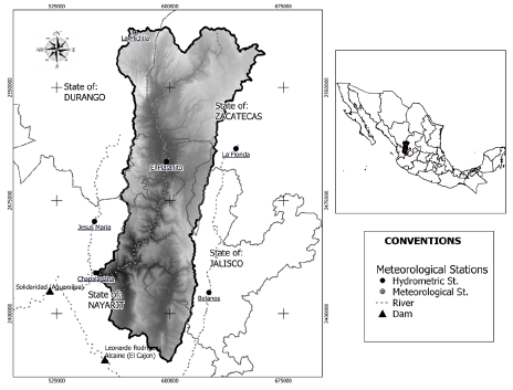
The Huaynamota River contributes to generating electricity. The Solidaridad dam (also known as Aguamilpa), located on the Lerma-Santiago River and geographically at 104°48'10,55" W and 21°50'22,74" N, produces 960 MW of electricity and has a maximum capacity of 5 540 million m3 of water (CONAGUA, 2008). The Huaynamota River discharges into the Santiago River, where the Aguamilpa dam is located, approximately 90 km upstream from the Pacific Ocean, into which the Santiago River empties on the coast of the Mexican state of Nayarit.
We implemented the EnKF (Evensen, 1994), DKF (Kalman, 1960), and ARX(1,1) (Bras and Rodríguez-Iturbe, 1985) algorithms. Forecasts were made at 1, 2, 3, 4, 5, and 6 h (L steps forward) of the flows at the Chapalagana station as a function of the flows at the Platanito station, located 100 km upstream from Chapalagana, as the exogenous variable. The hourly streamflow series between 9:00 hours on August 2 and 0:00 hours on September 28, 2017, were used, for a total of 1 360 registers supplied by Federal Electricity Comission (CFE).
EnKF, DKF, and ARX were implemented through R routines (R Core Team, 2021), which generate forecasts in six steps with DKF and ARX, and with 42 combinations between steps by set size in EnKF. Both EnKF and DKF were implemented to estimate the state vector corresponding to the response function of the basin, or Instantaneous Unitary Hydrograph (IUH) (Valdés et al., 1980). Values were estimated which correspond to the columns of the IUH. Multiplying these values by those of the measured series results in an estimation. In the three algorithms, the last observations of each series were considered (Valdés et al., 1980). The ARX model was recursively implemented based on a fraction of a series with 100 registers.
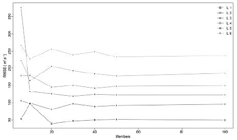
By means of the sensitivity analysis with 5, 10, 20, 30, 40, 50, and 100 members that were combined with the six steps, and based on the root mean square error (RMSE), the adequate number of members in the EnKF sets was determined (Quiroz et al., 2019). White noise that is integrated in the EnKF members was generated with the mvtnorm package (Multivariant Normal and t Distributions) (Genz and Bretz, 2009). In the evaluated Kalman Filter algorithms, the Q variance was assumed to be constant (Simon, 2001) with a value of zero (Morales-Velazquez ef al., 2014), and the R was assumed to have a near-zero value (0,01) in order to confer flexibility to the convergence of the algorithm (Welch and Bishop, 2006). With these values, the covariance matrices were created.
The fit reached by each algorithm was evaluated using the Nash-Sutcliffe coefficient (NS) (Nash and Sutcliffe, 1970) and the RMSE (Morales-Velázquez et al., 2014), as expressed by Equations (1) and (2). The assumed normality of errors was verified using graphs (González-Leiva et al., 2015).
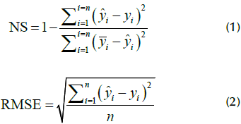
where y
i
is the forecasted data, y
i
is the observed data,  is the average of the observed data, is average of the forecasted data, and n is the amount of observations.
Ensemble Kalman Filter
To extend the functionality of the DKF (Kalman, 1960) and deal with non-linear dynamic systems, the EKF, among others, has been proposed (Jazwinski, 2007; Welch and Bishop, 2006), which includes the EnKF (Evensen, 1994, 2009). The EnKF emerges as an alternative to the EKF, which has a high computational demand (Evensen, 1994, 2009) and is a sub-optimal estimator that, via Monte Carlo simulations, estimates the statistical error (Evensen, 1994; Gillijns et al., 2006; Rafieeinasab et al., 2014). Errors should satisfy the normal distribution assumption and are estimated based on sets of q values.
The algorithm is based on two groups of equations: forecast and analysis (Figure 2). In this study, the cycle began with the forecast equations, using the random values that make up the first matrix X K ai thus obtaining the first forecast via the measurement equation. The error matrices of the forecast were calculated against the new measurement, which is the input for the analysis equations, where the states are updated as new measurements are entered.
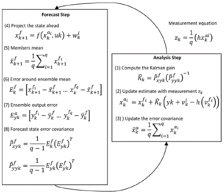
The h matrix is formed with the last register of two (n) hourly flow series of the Chapalagana and Platanitos stations. The uk parameter is absent because, in the upstream from the Chapalagana station, there are no structures (e.g., dams) that have a direct impact on streamflow. The errors v i k and v i k correspond to the noise contained by the process and the measurement, respectively. They are assumed to be white noise, with a mean of zero and variance Q and R (Figure 2). The noise in the measurements is generated by adding q deviations with normal distribution to the measurement in k time.
In the second analysis equation, the component y
k
+ v
i
k
represents the noisy measurements, у
к
is the measurement in time k, and the superscript i represents the number of members, i.e., random values under normal distribution that correspond to i = i,2,...,...,q. The adequate number of members in a set in hydrological studies is between 50 and 300 (Gillijns et al., 2006; Quiroz et al., 2019). The predicted value z
k
is obtained by averaging the vector resulting from multiplying the h matrix and the  and applying the measurement equation.
Discrete Kalman Filter
The DKF is an optimal recursive estimator of states in linear dynamic systems (Kalman, 1960) (Figure 2).
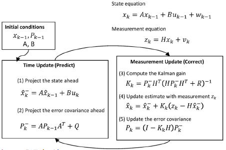
The state equation has two (n) hourly flow series from the Chapalagana and Platanitos stations. The matrices A (nxn) and В (n x 1) relate the state at time к - 1 to the current state at time k. Like the EnKF, the control matrix В is not included, given that, in the upriver from the Chapalagana station, there are no structures that have a direct impact on streamflow. Matrix A is assumed constant throughout the process, and matrix H is composed of a vector raw of 1 xn that contains the last observation of each entry series. The predicted value z k is obtained via the measurement equation by multiplying the H matrix by the state vector x k (n x 1).
Implicit in the predicted value z k is the measurement error w k - 1 and, likewise, the process error v k is contained in the state equation. In both cases, the normality assumption must be satisfied.
The state and measurement equations maintain a cycle that is repeated indefinitely. At time к - 1, it makes the a priori estimation (forecast) of the states, and, at time к they are updated (a posteriori estimation). The states are assumed to be the response function of the basin, and the a posteriori estimation corresponds to the forecast for time k+ 1. This cycle is repeated indefinitely, predicting time к + 1 based on the H matrix and the state vector updated to time k.
First-order autoregressive model
One of the first approximations for the forecast is the first-order autoregressive model, which is based on the autocorrelation that occurs within the same series of data (Box et al., 2016; Bras and Rodríguez-Iturbe, 1985). Algebraically, it is described as follows:
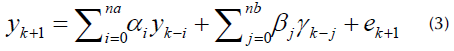
where y k+1 is the predicted value, α i and ß j are the model parameters, and y k and y k correspond to the entry variable and the exogenous variable, respectively. The parameters are estimated by the method of least squares, which requires a series section of at least 50 registers (Box et al., 2016; Shmueli and Lichtendahl, 2016). In the ARX(nα,nb) model, na and nb represent the autoregressive delays that are used in each variable.
Results and discussion
Forecasts with six-hour steps were made of the flows at the Chapalagana station. For the case of EnKF, seven set sizes were evaluated in order to estimate the error, which had 6, 10, 20, 30, 40, 50, and 100 members. Series with 1 360 registers were used, which included two main events.
As of 50 members per set, the EnKF algorithm showed a stable convergence for all steps. Consequently, under the conditions of this study, it is acceptable to use at least 50 members per set to have an adequate fit regarding the convergence of the algorithm and the stabilization of the error, aiming to minimize computational effort. As previously indicated, the results presented below have a base of 50 members per set. Table 1 presents the statistical indicators of fit for the observed series against the predicted one.
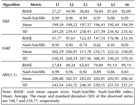
According to the statistical indicators in Table 1, the NS shows similarities between DKF and ARX, with values of 0,99 and 0,83 in steps one and six, respectively, while EnKF obtained 0,95 and 0,05 in steps one and six. According to the NS, the fit of all the steps is less with EnKF; in step one, it is 0,04 less, and there is a marked change up to step six, where the difference is around 0,78. The mean of the predicted series is more stable with DKF, followed by ARX and, finally, EnKF. EnKF and ARX show an upward trend in the mean value for each step, whereas DKF has a downward trend.
Despite the low fit values, the EnKF algorithm expressed the changes with a non-linear trend and showed better convergence on the observed series once it was updated with new measurements. DKF and ARX generated forecasts in which the displacement of the predicted series was accentuated against the observed series, similar to the persistent forecast method (Aguado-Rodríguez et al., 2016; Kavasseri and Seetharaman, 2009). This behavior is also noticeable in the work of Alvarado-Hernández et al. (2020), González-Leiva et al. (2015), and Morales-Velázquez et al. (2014).
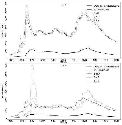
In the flood that began at 810 h, EnKF assumed the abrupt change in flow and generated a forecast with a steeper slope than DKF and ARX. Also, in the flow descents between 870 and 900 h, EnKF converged more precisely on the observed series (Figure 5).
Source: Authors
Figure 5 Observed flow and flows predicted with EnKF, DKF, and ARX (flood from 4/9/2017, 16:00 h, to 8/9/2017, 20:00 h)
The DKF fits are similar to those obtained by Alvarado-Hernández et al. (2020), who used the same series and a model that integrates ARX and DKF. This model considers the delay between series to be one, whereas, in our study, it was updated dynamically throughout the series, favoring the fit at peaks and reducing the effect of displacement of the predicted series. EnKF, in its six steps, obtained lower fits due to overestimation or underestimation at the peaks, with the difference that it achieved a better fit in ascents and descents of the observed series. The EnKF algorithm obtained a better temporal fit at peaks and converged more precisely on the observed series when the trend persisted in a number of hours higher or equal to the evaluated step.
The forecast with EnKF showed overestimations relative to the observed series. This occurred because we treated the measurements as a non-linear phenomenon (Evensen, 1994, 2009), a situation that, in step one, allows for an acceptable fit in the entire series. However, in step six, broad overestimations may be found which can affect the quality of the forecast. As the forecast step increases, the frequency of overestimations increases because the new register that serves to update the states also breaks away, and there may be changes in the L interval that are not considered in the initial forecast. The dynamic incorporation of the delay time between series (Meng et al., 2017) allows improving the fit, given that updating is performed with the equivalent event in the exogenous variable (Figure 6).
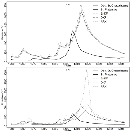
Source: Authors
Figure 6 Observed flow and flows predicted with EnKF, DKF and ARX (flood from 23/09/17, 10:00 h, to 28/09/17, 00:00 h)
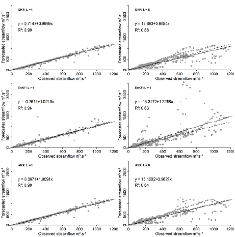
The dispersion of the observed series against the predicted one was congruent with the NS index, highlighting the similarities between DKF and ARX. The difference exhibited by EnKF is due to the peaks associated with abrupt changes in flow. The EnKF algorithm tended to overestimate throughout the series, unlike DFK and ARX, which caused a slight tendency to underestimate. Step six with EnKF produced large overestimations that are reflected as isolated points above the diagonal in Figure 7.
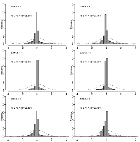
The standardized errors of the forecasts have a symmetrical distribution around zero (Figure 8) (Cryer and Chan, 2008; Martinez et al., 2012; Wang et al., 2017). According to Chatfield (2001), a behavior approaching normality is accepted. As shown in Figure 8, there is symmetry and higher concentration of registers in the central area of the Gauss bell curve. The proportion of registers between three standard deviations above and below the mean is more than 97%, and EnKF had the highest values in all steps.
As the steps of the forecast increase, the fit decreases, and overestimations and underestimations become more frequent for EnKF. Introducing coefficients that represent stationality and autocorrelation into the transference function can reduce the over-dimensioned estimations and achieve better fit.
Conclusions
The dynamic updating of delay time relative to the exogenous variable allowed improving the fit in the evaluated algorithms. The EnKF algorithm achieved a better convergence on the observed series but generated overestimations of greater magnitude as the step increased, which resulted in a lower degree of fit, as demonstrated with the Nash-Sutcliffe index. The potential of EnKF lies in its convergence and non-linear treatment of abrupt changes in flow. Basically, EnKF helps capture the non-linearity in some parts of the of the hydrograph and accurately represents the timing or times of occurrence of maximum flows, even though they are overestimated.
In future studies, the use of EnKF for streamflow forecasting can be a viable alternative when integrated with autocorrelation analysis, so that stationality and stationarity become part of the model, thus allowing to represent the changes associated with daytime, nighttime, or the months of the year. Together, the quantity of registers for updating the states can be increased in order to enable the detection of changes in trends during the last registered hours.
To improve the fit of the forecast, it is important to advance in research with step sizes of several hours (e.g., groups of six hours using the mean or maximum) in such a way that each step is equivalent to six hours and the forecast at six steps equals 36 hours.

