


 English (pdf)
 Article in xml format
 Article references
 Send this article by e-mail
 Cited by SciELO
  Cited by Google
  Similars in
SciELO
Similars in
SciELO  Similars in Google
 Permalink
Introduction
Water erosion, a soil degradation process also regarded as an environmental hazard (Mohammed et al., 2020; Duguma, 2022), is caused by precipitations falling on vulnerable bare terrain, which, as runoff across the slope, drag the soil along to finally deposit it in low areas or mire and obstruct bodies of water (Ávila and Ávila, 2015; Omuto and Vargas, 2019). This makes it the main soil degradation process, as it quantitatively and qualitatively affects the rootable volume of soils intended for agricultural production (Morales-Pavón et al., 2016) and contributes to the decline of many other essential ecosystem services (Chaudhary and Kumar, 2018; FAO, 2019).
A way to observe water erosion is through multispectral images captured via remote sensing. From this perspective, eroded soils are characterized by a spectral response similar to that of bare soils, i.e., much more uniform than that of vegetation, which exhibits a flatter reflectivity curve (Chuvieco, 2016), thus indicating the existence of bare soils or parent material outcrops as an effective indicator of areas subjected to erosion (Beguería, 2006). In light of the above, remote sensing techniques and geographical information system (GIS) procedures become necessary. These allow obtaining the spatial and temporal distribution of the diverse factors involved, along with their classifications (Rosales-Rodríguez, 2021). Thereupon, it is also necessary to perform visual and statistical analyses in order to understand and validate the generated cartography, whose purpose is to obtain a more precise and reliable cartographical indicator.
Some remote sensing techniques focus on visual quality by trying to improve the location of the data for analysis, in such a way that the features of interest are more evident (e.g., contrast expansion, color composition, and filtering) (Lillesand et al., 2015; Chuvieco, 2016). Other techniques aim to generate continuous variables, such as vegetation indices, which have proven to be efficient at evaluating soil degradation -with erosion among them (Ngandam et al., 2016)- by transforming them into Net Primary Productivity (NPP) values (Sartori et al., 2018), which has led them to be more frequently employed as quantitative indicators of ecosystem functioning (Orr et al., 2017). In the same way, they have been used to monitor vegetation in arid and semiarid lands (Najafi et al., 2020), as well as to generate the C-factor for models such as USLE (Universal Soil Loss Equation) (Meinen and Robinson, 2021).
Other techniques have also been created, such as i) soil indices (IS) used to estimate soil degradation types (Ngandam et al., 2016; Li and Chen, 2018); ii) principal components analysis (PCA) to discriminate types of bare soils or landslides (Romero et al., 2017; Basu et al., 2020); and iii) spectral mixture analysis (SMA) to map the C-factor or determine bare soils in order to construct vulnerability indicators (Demaría and Aguado, 2013).
In this sense, all these techniques may be used as steps prior to highlighting erosion and later allowing its semi-automatized classification in order to obtain a risk map (Duguma, 2022). These techniques also aim to overcome the tedious task of visually interpreting satellite images, as well as the considerable amount of time required to carry it out (Leal et al., 2018).
By making a special emphasis on erosion risk mapping, which usually indicates the relative probability of it taking place within a certain area as compared to others (Ganasri and Ramesh, 2016; Opeyemi et al., 2019), a distinction can be made between potential, defined as the maximum possible soil loss in the absence of vegetation cover and conservation practices (i.e., only considering the interaction between the physical factors of the soil: soil erodibility, rain erosivity, and topography), and actual, which is determined based on the sum of the land cover/use factor and the previous ones (Plambeck, 2020). The former tends to be substantially higher than the latter (Drzewiecki et al., 2014).
Therefore, the importance of remote sensing techniques to map erosion and its risk has become evident. In the same way, these methods have proven to be valuable for generating a cartography of soil degradation in climate change studies. This has been demonstrated in global products, such as soil degradation assessment (GLADA) (Anderson and Johnson, 2016); in regional ones, with erosion risk modeling in Europe (Panagos et al., 2015); and in national ones, with Malawi's atlas of soil loss (Omuto and Vargas, 2019). In the same way, some of these techniques have been used to monitor changes in cover or NPP and have been proposed within the analysis of land degradation neutrality (LDN) (Orr et al., 2017), whose sustainable development goal (SDG) for 2030 is to tackle desertification, rehabilitate degraded land and soil, and strive towards a world with "neutral soil degradation" (UNGA, 2015).
Identifying areas that have been eroded or are at risk of erosion also allows government agencies (via cross-referencing with population density maps) to initiate rehabilitation and protection activities, to perform territory planning for environmentally sustainable socioeconomic development, and to determine areas that are susceptible to hillslope processes (Ngandam et al., 2016; Efiong et al., 2021). Additionally, every action taken to address soil degradation may simultaneously contribute to the objectives of the fight against climate change, to the preservation of biological diversity, and to the SDGs (Orr et al., 2017).
In light of the aforementioned ideas, the main objective of this study was to map areas that are eroded and at risk of erosion using remote sensing techniques and GIS procedures, given that many models developed for this type of estimation cannot be adequately executed because data are missing to complete their parameters, e.g., soil erodibility, which requires properties such as structure and permeability, among others, which, in practice, are usually scarce or nonexistent for many parts of the world (Ávila and Ávila, 2015; United Nations, 2021). All results were obtained at a watershed located in a semiarid environment, a space where soils often stand out for their susceptibility to hydric erosion (Tsegaye et al., 2020).
Materials and methods
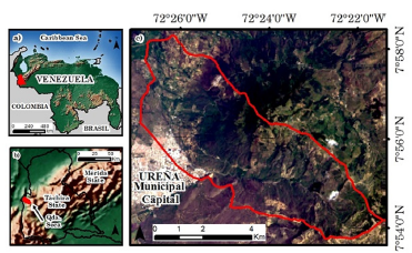
Study area: the studied watershed is located between the 72°26'43" - 72°21'23''O and 7°58'29" - 7°54'11"N. Its area is 37,31 km2 (Figure 1), and its altitude oscillates between 253 and 1 622 m.
Resources: the resources used for generating EAER and PWER are shown in Table 1.
Table 1 Resources
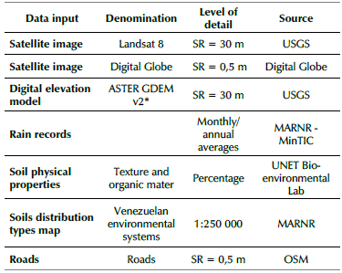
*ASTER Global Digital Elevation Model 2; SR: Spatial Resolution -USGS: US Geological Survey; MARNR: Ministry of the Environment and Renewable Natural Resources; MinTIC: Ministry of Information and Communication Technologies; OSM: Open Street Map.
Source: Authors
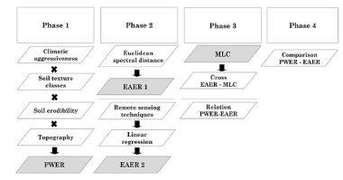
General methodology: a systematic scientific literature review was carried out to identify a deterministic PWER (potential water erosion risk) model, remote sensing techniques, and GIS procedures, with the purpose of identifying eroded areas and areas at risk of erosion (EAER). Four main phases were implemented: 1) developing the PWER model, 2) obtaining the EAER, 3) evaluating the degree of accuracy regarding the EAER with a supervised maximum likelihood classification (MLC) and a comparison of PWER and EAER, and 4) analyzing the results (Figure 2).
Landsat 8 OLI/TIRS image processing: a satellite image from October 1, 2017, was downloaded (LC08_L1TP_00705 5_20171001_20171013_01_T1_sr) with surface reflectance values and L1T corrections (IGAC, 2013), as well as topographic correction performed by Camargo et al. (2021).
Digitai Globe image: a natural color image from May 7, 2018, was employed. It had a spatial resolution of 0,5 m (SIGIS, 2019) and was supported by Google Earth, which allows its use in non-profit research (Thenkabail, 2016). Said image aided in the selection of 'ground-truth' samples in order to increase risk prediction reliability, based on a qualitative approach of erosion severity classes (Auerswald et al., 2018; Fischer et al, 2018; Batista et al., 2019).
PWER methodology
This methodology is based on two principles. The first one of a fundamental nature, expresses that it is the land that suffers the attack of the forces of climate (climatic aggressiveness) and that it, in turn, offers variable degrees of resistance, which poses a relation that determines the degrees of degradation in a given area. The second one indicates that potential risk assessment is most useful when relatively unstable or non-permanent factors (vegetation and land use) are not included in the calculation (FAO et al., 1980). Recent studies that use these principles include, among others, Guerra et al. (2020), Allafta and Oop (2021), and Al-Mamari et al. (2023). The PWER manifests via Equation (1):
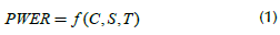
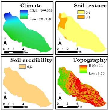
PWER is expressed in Mg ha-1year-1; C is the rain erosivity factor; S is the soil factor, estimated by means of texture (st) and erodibility (se) subfactors; and T is the topography factor (FAO et al., 1980; Rosales and García, 2015).
The climate factor (C) was evaluated based on the modification of the Fournier index (1960) (Arnoldus, 1977), which is best correlated with the EI30 value (maximum rain intensity in mm-hr-1 with 30 min duration), which has been verified in several parts of the world and is regarded as valid for Venezuela (Pacheco, 2012). The original Fournier index was not employed, as it does not consider that there are areas whose rainfall regime may have more than a monthly precipitation peak (Muñoz et al., 2014). Then, interpolated monthly precipitation surfaces were generated using IDW (inverse distance weighting) instead of kriging, as not all assumptions for its use are fulfilled (Hämmerly et al., 2019).
The S-factor was estimated based on st and se features associated with a soil type distribution map (MARNR, 1983) given the scarce availability of detailed soil data, which generally leads to considering reconnaissance studies (Quiñonez and Dal Pozzo, 2008). The texture classes of the first ones were conformed (USDA, 2020) and reclassified into three general categories recognized by FAO-UNESCO (1976), which in turn allowed assigning the valuations necessary for the model as per FAO et al. (1980). As for the second ones, the nomogram of the USLE K factor was employed (Foster et al., 1981 ), which is between 0 and 0,09 Mg ha h / ha MJ mm, using organic matter and texture percentages, later associated with erodibility values and classes and valuations as per FAO et al. (1980).
Finally, the T-factor was obtained from the ASTER GDEM, in which three slope classes were distinguished: a) flat to mildly undulating (0-8%); b) strongly undulating to hilly (8-30%); and c) strongly eroded to mountainous (>30%) (FAO-UNESCO, 1976), which were rated at (a) 0,35; (b) 3,5, and (c) 11,0 (FAO et al., 1980).
EAER methodology
Two mapping alternatives were developed: the first one was based on the spectral Euclidean distance between the reflectivity of each pixel in the satellite image and the bare soils category, and the second one on diverse remote sensing techniques, with which linear regressions were established. ROC (receiver operating characteristics) curves were applied to both products, which allowed defining classification thresholds and associated uncertainties aimed at detecting similar contiguous spectral zones of eroded and erosion risk areas (Beguería, 2006; Alatorre and Beguería, 2009). For thresholds, 100 independent samples (pixels) were selected, which evidenced <10% of vegetation cover, randomly distributed and defined with the help of the Digital Globe image, as the risk of erosion is considered to be high when this value is low (Wang et al., 2021).
An ROC curve is a graph that incorporates all sensitivity/ specificity pairs resulting from the continuous variation of cutoff points throughout the range of observed results. This offers a global view of diagnostic accuracy by providing significant data on the probability of correctly classifying an individual by means of a determined variable (Ampudia et al., 2017). Their equations are:
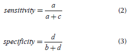
where a are true positives, b true negatives, c false positives, and d false negatives. Sensitivity expresses the proportion of correctly predicted positive pixels, and specificity represents the proportion of correctly predicted negative pixels.
Sensitivity and specificity values of 1 represent the likelihood of omission (type II, or false negative) and commission (type I, or false positive) errors (Alatorre and Beguería, 2009). In order to determine eroded areas, a sensitivity value of 0,9 was fixed, which corresponds to a 10% probability of omission errors. For areas at risk, a value of 0,8 was set (20% probability of omission error).
A supervised maximum likelihood classification (MLC) of the covers was carried out, as it is more precise than an unsupervised one because its classes are previously known (Liang and Wang, 2020). This, to later evaluate accuracy at determining bare soil cover with EAER by means of cross-tabulation. These results were updated with highways (OSM) and validated via global precision (Chuvieco, 2016) and kappa statistics (Cohen, 1960).
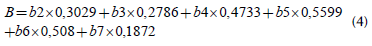
The remote sensing techniques implemented were vegetation indices based on slope and distance, soil indices (equations in Table 2), and others such as principal components analysis (PCA) (Pearson, 1901), spectral mixture analysis (SMA) (Boardman, 1992) and tasseled cap brightness (B) (Kauth and Thomas, 1976), with the coefficients derived by Baig (2014) for Landsat 8 Oli, as shown in Equation (4):
Then, a linear regression analysis was carried out in order to determine the degree of dependence present between two variables (Shobha and Rangaswamy, 2018). To this effect, the bare soil spectral Euclidean distance was considered as an independent variable (x) and each technique as a dependent variable (y). Correlation tests were conducted in order to show the degree of the linear relation. Finally, all p-values generated were lower than 0,001, taking into account that values lower than 0,05 had to be considered in the analysis.
The resulting maps show three categories: (i) eroded areas, understood as those with no vegetation and denoting active erosion; (ii) at risk areas, those with little vegetation and prone to erosion; and (iii) no erosion, areas with good vegetation cover that 'apparently' protect against erosion.
Results
PWER
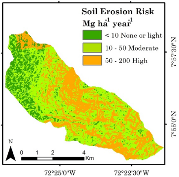
The behavior of the factors (Figure 3) allows defining a C-factor between 78,94 and 106,65. S was defined as fine (0,1) and medium (0,3) in terms of subfactor st, and as light (0,5) in terms of subfactor se (Table 3). T was between 0,35 and 11. Once the variables were defined, they were multiplied in map algebra in order to obtain PWER and later reclassify it to establish the soil erosion risk classes (Figure 4), thus obtaining 542,07 ha for 'none to light' (14,59%), 1 805,76 ha for 'moderate' (48,60%), and 1 767,37 ha for 'high' (36,80%).
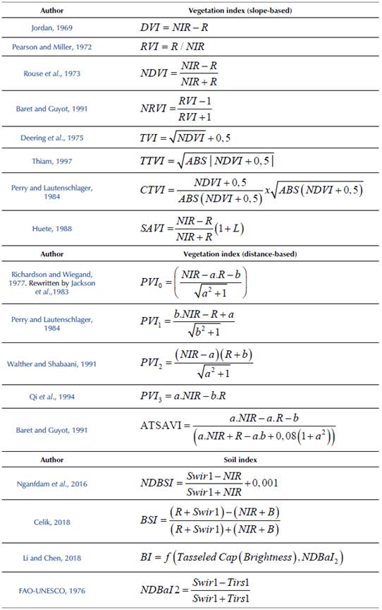
Table 3 Soil subfactors processing
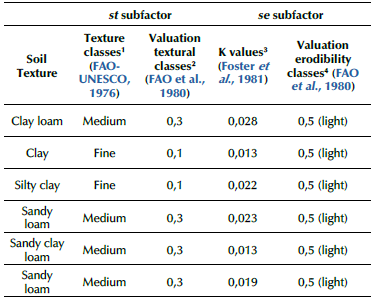
1 Soil texture classes: coarse: <18% clay & >65% sand; medium: <35% clay & < 65% sand 0 < 18% clay & <82% sand; fine: >35% clay
2 st Classification: coarse: 0,2 medium: 0,3 fine: 0,1 stony phase: 0,5
3 K-value: light: <0,03; moderate: 0,03-0,06; high: 0,06 >.
4 se valuation: light: 0,5; moderate: 1,0; high: 2,0.
Source: Authors
Maximum likelihood classification (MLC)
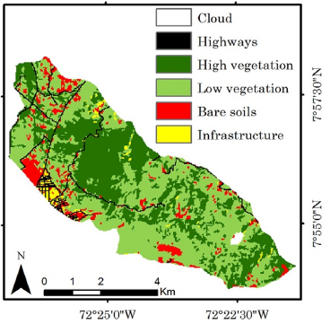
Six categories were established, and their areas were extracted: clouds (13,95 ha), highways (163,98 ha), high vegetation (1 331,10 ha), low vegetation (1 874,07 ha), bare soils (including rocky outcroppings) (277,74 ha), and infrastructure (69,36 ha) (Figure 5). The map had a global accuracy of 81,83% and a kappa index of 0,79.
EAER1
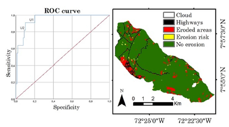
The ROC curve showed a high sensitivity, i.e., good capabilities to correctly classify positive pixels (bare soils). The 0,9 (U1) and 0,8 (U2) thresholds indicated spectral distances of 0,114 and 0,087. Both represent a balance between sensitivity and specificity. That is to say, an approach to the most ideal conditions (100%), which allowed generating the map (Figure 6) with the following results: eroded areas: 379,44 ha; erosion risk: 260,91 ha; no erosion: 2 911,95 ha (Figure 6).
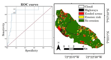
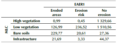
Cross-referencing with MLC indicated that the eroded areas coincided with 229,77 ha of bare soils. In the same way, this category intercepted 'high vegetation' in 0,99 ha, 'low vegetation' in 126,99 ha, and 'infrastructure' in 21,69 ha. For its part, the erosion risk class mainly intercepted 'low vegetation' (236,52 ha), 'bare soils' (20,61 ha), 'infrastructure' (3,33 ha), and 'high vegetation' (0,45 ha) (Table 4).
EAER2
Once the products of the remote sensing techniques were derived, linear regressions were carried out. The analysis showed that the slope value was different from 0 in all cases, i.e., there is a dependence between the variables. Under this criterion, SAVI is the most dependent (2,75), as it has the most inclined line, with a direct (positive) dependence, followed by NDVI (1,83) (Table 5).
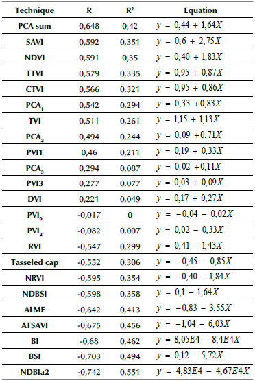
By only analyzing the correlation coefficients (R), the highest results were obtained by SAVI (0,592), NDVI (0,591), TTVI (0,579), CTVI (0,566), and PCA1 (0,542). Nevertheless, all of them were surpassed by the PCA sum, which achieved a value of 0,648. As for the R2, it was found that only the PVI0 showed a value equal to 0, which means that it does not explain any variation in this index as a function of the independent variable. It is closely followed by PVI2 and DVI, which may be explained by their low correlations.
Among all the implemented techniques, NDBIa2 is the one that is most determined by the spectral Euclidean distance of the soil, with an R2 of 0,551. However, it also showed the highest negative correlation (-0,742). Similar situations were reported by BSI, BI, and ATSAVI. On the contrary, the technique with the best R2 was the PCA sum (0,420), as it showed a positive correlation of 0,648 (the highest one), which makes it the second EAER alternative.
Then, an ROC curve was elaborated based on 100 samples of PCA sum values. The 0,9 (U1) and 0,8 (U2) thresholds indicated values of -0,117 and -0,107 for the PCA sum, respectively, which represent a good balance between sensitivity and specificity, thus allowing to generate the map (Figure 7) with the following results: eroded areas: (261,18 ha); erosion risk: 25,83 ha; no erosion: 3 265,29 ha.
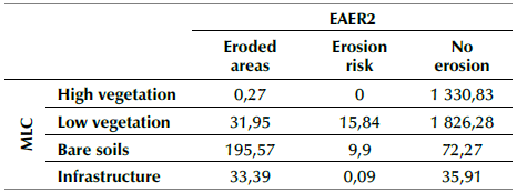
Cross-referencing with MLC indicated that the surface occupied by eroded areas coincided with 195,57 ha of bare soils and intercepted 'high vegetation' in 0,27 ha, 'low vegetation' in 31,95 ha, and 'infrastructure' in 33,39 ha. For its part, 'erosion risk' intercepted 'low vegetation' in 15,84 ha, 'bare soils' in 9,9 ha, and 'infrastructure' in 0,09 ha (Table 6).
With the purpose of understanding the PWER as an indicator of erosion sensitivity, 14 bare soil pixels (samples) were first analyzed (Figure 8) based on the relationship between the thematic categories defined for the EAER, the classification by FAO et al. (1980), and the PWER values (Table 7). It must be highlighted that, given that the samples of bare and erosionexposed soils were identified based on a higher-resolution image, they should only be classified as eroded or erosion risk areas in the EAER ('no erosion' would be an imprecision generated by the change in spatial resolution or threshold definition). Secondly, the possible soil loss quantities were totalized for eroded and erosion risk areas, with the purpose of evidencing the approach with the most losses.
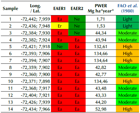
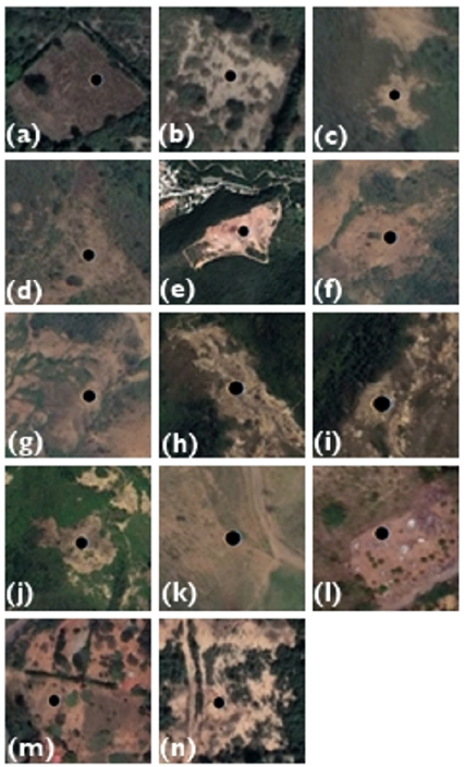
The results allowed defining a higher success rate in EAER1. However, an imprecision was found in sample 5, which was considered to belong to 'no erosion' (Figure 8e), as it is completely uncovered. This was the only incongruence generated in EAER1, since the correct category should have been 'eroded areas', i.e., spectral distance values lower than 0,087. For its part, EAER2 showed three contradictions when it categorized samples 1, 2, and 3 as 'no erosion', even when they were uncovered (Figures 8a, 8b, and 8c). These pixels should have been lower than the PCA sum value of -0,107 (incongruences refer to values lower than those established by the thresholds in the ROC curves).
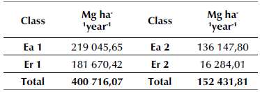
Considering the high success rate of the samples in both EAER, the PWER condition of the 14 points could be observed. In the case of sample 5 in EAER1, potential degradation is considered to be high, with 132,61 Mg ha-1year-1. On the other hand, sample 3 in EAER2 showed a loss of 44,34 Mg ha-1year-1, which represents a moderate degradation (the remaining samples can be interpreted in the same way). Finally, the soil losses from eroded and erosion risk areas in the first map were much greater than those of the second (by 162,88%) (Table 8).
Discussion
Even though the PWER methodology dates back to 1980, it is still valid because its application is ideal when there is no adequate information on precipitation, evapotranspiration, lithology, and soils, which is required by methodologies such as USLE or the one proposed by Pacheco (2012) or more recently by Nasir et al. (2023). On the contrary, the need for minimal information such as monthly precipitations, free MDE, and reconnaissance-level soil mapping provides this methodology with execution plausibility, simplicity, and scientific robustness. It is also important to note that many of the models currently used require the inclusion of impractical variables (Demirel and Tüzün, 2011), which highlights the need for new approaches in the modeling of erosion processes (Nasir et al., 2023).
A case that illustrates the above is the comparison between the potential erosion results obtained in this study and those of Condori-Tintaya et al. (2022) and Nasir et al. (2023).
While the former used soil structure information and calculated a more complex length and slope factor based on equations, the latter employed a multi-criteria decision making (MCDM) approach involving the development of 15 variables and an analytical hierarchy process (AHP).
Access to GIS and satellite images has had great impact on erosion modeling. Models can now be applied with relative ease at a large scale and in a distributed fashion, and they can present results in pixels that allow identifying where they occur and their magnitude, as well as at different temporal and spatial scales (Batista et al., 2019). However, it is also recognized that the predictive capability of large-scale erosion models is not the best. Therefore, Alewell et al. (2019) have argued that the same should not strive for them to make accurate predictions of soil losses, but instead to explore scenarios and focus on understanding relative differences in erosion rates, which would help to identify areas prone to these degradation processes, which is the objective of this study.
In the same way, very high-resolution images may be used to test erosion models, which has not been widely performed by researchers, with Fischer et al. (2018) perhaps being the first to focus completely on its interpretation. They found promising results, such as a high correlation (R2= 0,91) of visually defined erosion classes with moderate soil losses, thus allowing them to define a semi-quantitative assessment approach, which is much simpler than proposing hypothesis tests (Batista et al., 2019).
Other reasons to support the use of this methodology is that it excludes speculations on the validity of the models' predictions, and it allows identifying scenarios leading to great or small soil losses (Auerswald et al., 2018). This study did not employ a semi-quantitative approach because the real soil loss values of the samples selected were not calculated independently, so as to be able to determine the R2, which denotes a predominantly qualitative assessment to address comparative analyses.
The key to proceeding with the identification of EAER lies in the accurate extraction of vegetation cover and land use (Wang et al., 2013). In this case, it involved aiming for the highest possible accuracy regarding bare soils, with which the spectral Euclidean distance was obtained to later define thresholds in ROC curves, since the presence of vegetation cover reflects resistance capabilities against erosion or its risk (Wang et al., 2021).
Starting with 'eroded areas' and its intersection with bare soils (379,44 ha = 100%), cross-tabulation between MLC and the EAER allowed corroborating that there was a higher intersection in EAER1 (60,55%) in comparison with EAER2, which coincided by 51,54%. This result evinces the former's greater reliability, which is very likely due to the not-so-high correlation and determination coefficients of the PCA sum with respect to the spectral Euclidean distance.
As for the cross-reference between 'eroded areas' and 'low and high vegetation', EAER1 showed a 3,43% coincidence, unlike EAER2, which reported 0,87%. The intersection between 'eroded areas' and 'infrastructure' was lower in EAER1, with 0,58%, in contrast with the EAER2's 0,90%. These results are also explained by the differentiation inability shown by the latter, which is due to the not-so-high correlation and determination of the PCA sum.
These results position EAER1 as a baseline alternative in contrast with the PCA sum. This conclusion is reasonable, as this input was used as an independent variable in linear regressions.
As for the selection of thresholds in ROC curves, given the varying sensitivity/specificity, other thresholds with more or less discrimination power could be selected. Selecting two with a high sensitivity would reciprocally allow achieving a high probability of correctly classifying a pixel whose real situation is defined as positive. The advantage of the ROC curve lies in the fact that it uses all possible cutoff points in the database, through which better thresholds are determined, thus indicating that this test has a very useful and correct classification power (Bernui et al., 2022).
Therefore, the proposed method for identifying EAER differs from associating higher loss values (Mg ha-1 year-1) yielded by USLE and/or similar models as an indirect measure of diverse erosion risk degrees (e.g., Chaudhary and Kumar, 2018; Mohammed et al., 2020), which is supported by the assumption that low values are less vulnerable and high values refer to a greater erosion sensitivity (Meshesha et al., 2012). This also contrasts with the idea of obtaining them by ranking and later zoning, which results from intersecting diverse slope gradients from an MDE or land uses with soil losses (Meshesha et al., 2012; Khosrokhani and Pradhan, 2013; Wang et al., 2013).
The equivalence between remote sensing techniques obtained by linear regression was manifested by Ngandam et al. (2016), who proposed a vegetation index as the independent variable, which placed an exaggerated reliability in said product as a predictor. This, unlike the design implemented in this study, which was defined based on the spectral distance of bare soils.
The comparison between the qualitative and the quantitative results allows establishing a bidirectional complementary analysis relationship. In the first place, EAER helped to identify areas with erosion or highlight those at risk, in which soil losses can be interpreted. Secondly, it allows establishing the inverse relationship, i.e., the observation of possible high and moderate losses identified by the PWER provides information on what happens in said areas from a qualitative perspective.
For a wider understanding and for determining the possible existence of erosion or of areas that might be subjected to it, it is suggested that eroded and erosion risk areas be identified with both mappings. This consideration is supported by the identification of possible substantial differences at potential points of interest.
Finally, based on the study by Batista et al. (2019) regarding the fact that the current, different erosion models do not systematically surpass each other, this research agrees that calibration is the only mechanism to improve their performance (i.e., a better conceptual understanding of their operation). Therefore, this study rejects the notion that these can be validated (rather than evaluated), stressing the need to define adjustment tests (or evaluating degrees of reliability) based on multiple data sources, which allow for a wide study of the usefulness and consistency of the developed methodologies. This, considering that the more thorough the tests, the more likely it is that deficient performances are found (critical awareness of the methods).
Conclusions
Using remote sensing images allows conducting research on erosion both qualitatively and quantitatively. However, these must be used with care, as their unthinking use may lead to over- or underestimation. The use of very high-resolution images must also be considered as a mechanism to evaluate model performance.
Resorting to higher resolution imagery or covering larger extensions implies a higher computational cost because it involves larger amounts of data. This could be overcome by using cloud computing platforms such as Google Earth Engine (GEE), which can compute and process large volumes of geospatial data in very short time intervals and have been recently applied to the preparation of the variables required by methods such as USLE and RUSLE (Papaiordanidis et al., 2019; Kumar et al., 2022), so their application with the models developed in this study is also plausible.
Although technological advances are evident, it should not be forgotten that erosion models are not necessarily true or free of apparent flaws; recognizing them improves the attitude towards evaluating them and changes the way their performances are characterized and communicated, ultimately leading to a better understanding of soil erosion (Batista et al., 2019).
This study constitutes a contribution to the lack of precipitation and soil data, which is necessary in parametric methodologies. Therefore, it adopted the premise that this lack should be only resolved with free and available digital inputs that help identify potential erosion hot spot areas and simulate erosion responses to land use and climate change, which makes it a solution that could be associated with variables derived from MDE (e.g., humidity indices) or other kinds of categorical or continuous mapping. Nevertheless, regardless of the methods to be employed, an on-field survey of geo-referenced measurements (when possible) regarding erosion characteristics must not be discarded, with the purpose of broadening the model's evaluation.
Even though it is true that the methods developed for identifying EAER are metric-static and implemented with satellite images from diverse dates, these could help to obtain time series allowing to better understand the dynamics of erosion processes and therefore acquire greater knowledge for soil conservation and ecosystem management. They could also be replicated in other spaces in a semi-automatized fashion, and they could serve as first inputs to define areas where observations should be focused or to map types and degrees of erosion.

