


Services on Demand
Journal
Article
 English (pdf)
 Article in xml format
 Article references
 Send this article by e-mail
Indicators
-
 Cited by SciELO
 -
 Access statistics
Related links
-
 Cited by Google
 -
 Similars in
SciELO
Similars in
SciELO -
 Similars in Google
Share

 Permalink
Revista Facultad de Ingeniería Universidad de Antioquia
Print version ISSN 0120-6230On-line version ISSN 2422-2844
Rev.fac.ing.univ. Antioquia no.51 Medellín Jan./March 2010
CFD Numerical simulations of Francis turbines
Simulación numérica (CFD) de turbinas Francis
Santiago Laín1*, Manuel García2, Brian Quintero1, Santiago Orrego2
1Grupo de Investigación en Mecánica de Fluidos. Universidad Autónoma de Occidente, Calle 25 No 115 - 85 Kilómetro 2 Vía Jamundí Cali, Colombia
2Grupo de Investigación en Mecánica Aplicada. Universidad EAFIT, Carrera 49 - 7 Sur 50 Medellín, Colombia
Abstract
In this paper the description of the internal flow in a Francis turbine is addressed from a numerical point of view. The simulation methodology depends on the objectives. On the one hand, steady simulations are able to provide the hill chart of the turbine and energetic losses in its components. On the other hand, unsteady simulations are required to investigate the fluctuating pressure dynamics and the rotor-stator interaction. Both strategies are applied in this paper to a working Francis turbine in Colombia. The employed CFD package is ANSYS-CFX v. 11. The obtained results are in good agreement with the in site experiments, especially for the characteristic curve.
Keywords: CFD, turbulence, Francis turbine, steady and unsteady simulations
Resumen
En este artículo se aborda la simulación numérica del flujo en el interior de una turbina Francis. La metodología a seguir para la simulación del flujo en una turbina Francis depende de los objetivos perseguidos: mientras que para determinar la curva característica y las pérdidas de energía en los diferentes componentes basta una aproximación estacionaria, para investigar las interacciones rotor - estator o las fluctuaciones de presión en el rodete se requiere realizar un cálculo transitorio. Ambas estrategias se presentan en este artículo aplicadas a una turbina Francis en explotación en Colombia. La simulación se realiza por medio del paquete computacional Ansys CFX v. 11. Los resultados de la simulación comparan satisfactoriamente con las medidas experimentales realizadas sobre la máquina, especialmente en el caso de la curva característica.
Palabras clave: CFD, turbulencia, turbina Francis, simulaciones estacionarias y no estacionarias
Introduction
Hydroelectric energy is a clean, renewable energy as it only requires water. The machines that convert the energy into electricity are the hydraulic turbines, which are produced since many years ago. For this reason, the technology of such turbomachines is quite well developed, reaching mechanical efficiencies over 95%. However, reaching such efficiencies is a complex task and requires a high engineering effort because hydraulic turbines are usually unique products which must be designed for determined local conditions (head and discharge). For this reason, a specific design for each component of the machine is needed. The traditional design process is based on experiments, measurements and model tests, which implies important money and time investments. During the last 20 years the numerical simulation of the flow or Computational Fluid Mechanics (CFD) has been adopted as an additional element in the design process allowing to shorten the development times and saving money [1-4].
Moreover, in the hydroelectric industry, small improvements in the geometry of rotating elements of a hydraulic turbine can have a large positive effect from the point of view of operation and maintenance costs. However, in order to identify such improvements in the first stages of the design process, it is needed to consider all the components and interactions between them. The optimisation process based on simulations consists of an advanced CFD simulation software package coupled with a CAD environment. This coupling is critical in the preliminary designs because it helps to detect possible problems and to find the fastest way to optimise the machine.
The first step in any CFD simulation is to build the geometry model that represents the object to be modelled. Therefore, it is needed to generate a grid (figure 1, top) where are located the cells or control volumes. After the grid is finished, the boundary and initial conditions must be specified. The software solves then the fluid flow governing equations for each cell up to an acceptable convergence is achieved. When the model has been solved, the results can be analysed numerically and graphically (figure 1, bottom).
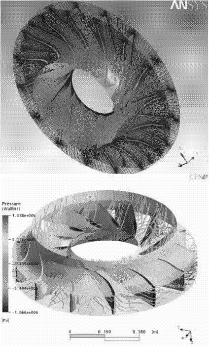
Figure 1 Computational grid (top) and pressure distribution (bottom) on the runner blades of a Francis turbine
In fact, during the last years, with the fast development of computational technology and advanced CFD, the internal flow simulation in individual or several components of a hydraulic turbine has became nearly a routine task [5-7]. Nevertheless, the flow in a hydraulic turbine is extremely rich and complex because the flow is usually turbulent, unsteady, with high pressure gradients, probably two phase (water - air) and highly three-dimensional (3D) with strong effects of curvature and rotation. Due to all these reasons, the numerical simulation and prediction of the flow in such machines is a highly demanding task with many difficulties.
A specific situation of the hydraulic turbines happens by the variable energy demand of the market, which means that the economic benefit depends frequently of the efficient operation at partial loads, far from the optimum design conditions. However, Francis turbines at partial loads present a very strong vortex, the so-called vortex rope, at the rotor exit. As the rotating flow is slowed down at the draft tube, a hydrodynamic instability appears in which the vortex rope changes its position periodically generating strongly unsteady pressure fluctuations in the draft tube walls, which may lead to material fatigue failure after long times. This phenomenon is particularly severe when the oscillation frequency of the vortex rope is coupled with the resonant frequency of the turbine or the hydraulic circuit. As it is usually not possible, or at least cheap, to measure the vortex rope behavior in operating turbines, the numerical simulation is an alternative to obtain the frequency, intensity of the pressure pulses and other parameters for several geometries and operating conditions of the turbine. Such information allows optimizing the turbine design to reduce the vortex rope strength and diminish the pressure fluctuations reducing the risk of material fatigue failure. Nevertheless, to compute these dynamic effects it is compulsory to perform an unsteady flow simulation, including all the interactions between components. Moreover, due to the non-uniformity of the flow at the spiral case exit and the different positioning of the wicket gates and runner blades it is needed to consider the full turbine, without any simplification due to rotational symmetry, with a fine enough grid. Nowadays, such simulation is out of the bounds of the computational power. For this reason, in the literature is common to include simplifications in the unsteady simulations.
Simulations methodology
Due to the complexity of the internal flow in a Francis turbine, the machine is usually divided in its components: spiral case (SC), stay vanes (V), guide vanes (O), runner (B) and draft tube (D). Such components are illustrated in figure 2 (top) and, schematically in a transversal cut, in figure 2, bottom.
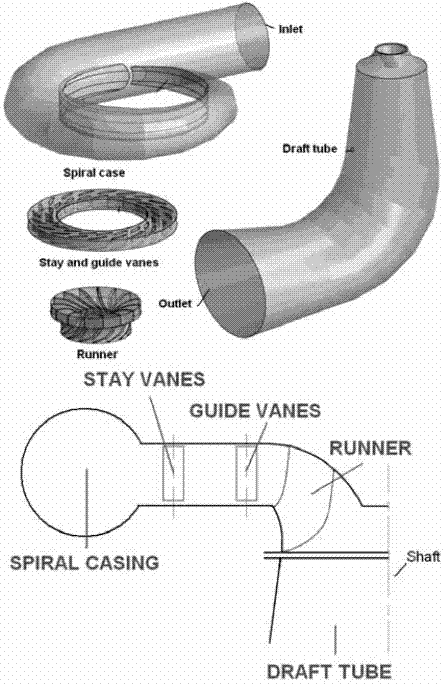
Figure 2 Scheme of a Francis turbine. Components (top) and transversal section (bottom)
The type of simulation to be performed on a Francis turbine as well as the methodology is determined by the results and variables sought. Specifically, four types of simulations can be distinguished in Francis turbine: 1. Hill chart determination; 2. Losses analysis (efficiencies) in different components; 3. Rotor-stator interaction analysis; and 4. Pressure fluctuations in the runner. This work is focused on the first (steady simulation) and third (unsteady simulation) types.
The ideal simulation aimed to predict all the relevant phenomena in a Francis turbine would be an unsteady simulation considering only one domain composed by all the components. Unfortunately, this ideal simulation is still far from nowadays computational capabilities due to the complexity of the grid generation and to the extremely high number of cells needed (estimated around 7 million). Moreover, the computational cost for unsteady simulation is much more higher than for the steady state simulations, of the order of 10 to 100 times more [8].
Therefore, the strategy consists of performing a separate grid for each component, controlling its number of cells, refining the grid locally in the most sensible zones and caring about the quality of the grid. The computational domains needed for the simulation of the flow inside the turbine are: the spiral case, the wicket gates (fixed and guide vanes), the runner and the draft tube, which are illustrated in figure 3. Each component was previously modeled through different reconstruction techniques and laser scan from the original turbine.
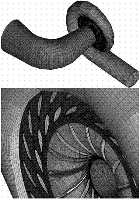
Figure 3 Top: geometric model of the Francis turbine considered in this study. Bottom: detail of the structured grid showing the respective domain assembly
For the steady simulations, with the purpose of obtaining a good enough accuracy in the zones where the variable gradients are high and keeping moderate the number of cells needed, the ideal simulation of the Francis turbine is divided in two or even more sequential simulations. Each CFD simulation has a different methodology aimed to obtain more accurate results. In this way it is feasible to perform simulations with roughly 2 million cells, which allow describing in detail the most relevant phenomena taking place in the turbine in steady state. Moreover, the minimum grid requirements for describing the boundary layer development can be adequately reached.
Table 1 shows the steady simulation partitioning aimed to obtain accurate enough results, taking into account the number of blades and the required grid density. The simulation 1 is focused on the accurate description of the flow inside the spiral case and it is aimed to provide a good inlet conditions to simulation 2. On the other hand, simulation 2 pretends to reproduce, with enough detail, the flow in the runner and the draft tube. For such reason, it only considers a part of the total domain respecting the rotational periodicity of the guide vanes and runner blades (i.e., 4/3). In this way, it is possible to numerically calculate the hydraulic losses and the hill chart of a Francis turbine, overcoming the computational restrictions of the size and quality of the required grids.
Each of this two simulations considers a steady state, because the description of unsteady phenomena is not pursued, allowing a significant computational saving. The simulations were performed with the CFX v. 11 software package. This software is based on the Finite Volume Method and solves the incompressible Navier- Stokes equations temporally averaged (RANS) in their conservative formulation (conservation of mass, momentum and energy). The system of equations is closed with two additional equations of the Shear Stress Transport (SST) turbulence model [9]. The equations are discretised by an advective high resolution scheme. The adopted convergence criteria for the RMS residuals of pressure and velocity has been 10-5 in all the simulations.
To perform the grid independency study, table 2 presents a summary of the generated grids for the turbine components of each simulation, indicating the number of cells in each part.
Table 1 Types of simulations
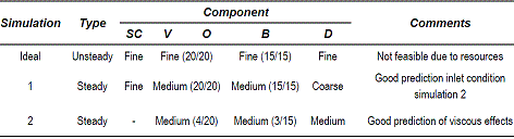
Table 2 Summary of generated grids
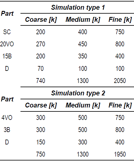
It can be seen that for the fine grid simulations the total number of cells is around 2 million, a feasible number for the available computational resources.
Moreover, in order to evaluate the sensibility of results versus the grid size, a study on grid independence was carried out. The reference value was the mechanical torque generated on all the runner blades plus that on the hub and shroud surfaces. Figure 4 shows that a grid of roughly 1300000 cells allows to obtain torque values virtually independent of the number of cells. The presented case in the figure corresponds to the nominal operation point with a volumetric flow of 4.8 m3/s generating approximately 10 Mw. Therefore, with the purpose of obtaining valid results of the steady CFD simulations using the minimum computational resources and capturing the relevant hydraulic phenomena, the medium grid was selected.
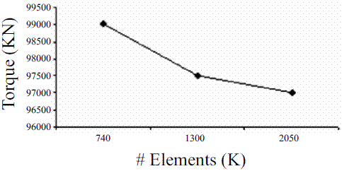
Figure 4 Dependence of torque versus grid size
On the other hand, the present objective of the unsteady simulations was to capture the rotorstator interaction phenomena, by obtaining the pressure fluctuation signals in several fixed points, which are later processed by fast Fourier transforms (FFT) in order to determine their intensity and characteristic frequency. However, the nature of the rotor-stator phenomena prevents of partitioning the simulation, so it was necessary to consider the full machine with a total number of cells around 2 million.
As the steady simulations, the unsteady simulations were also performed with the commercial software ANSYS CFX 11®, with the same characteristics of discretisation and turbulence model. The time discretisation of the equations was realized with the implicit second order Backward Euler scheme and for a time step corresponding to the time needed for the runner to rotate 1 degree (1.85x10⁻⁴ s) following recommendations of Vu et al. (2004) [10]. Each unsteady simulation was run for a time equivalent to 30 runner revolutions.
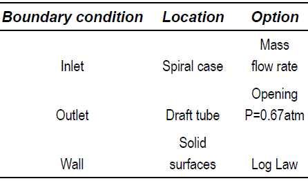
The employed boundary conditions for the steady and unsteady simulations were the same. The mass flow was specified at the inlet. In the outlet the opening condition with the specified pressure was used. This kind of boundary was the appropriate one for representing the actual conditions in which the real turbines operates. The solid surfaces were selected as walls. Table 3 summarises such boundary conditions in the simulations.
As the simulations are based in the Multiple Frame Reference concept, the interfaces between rotating and non-rotating components of the machine must be specified. Therefore, in the steady simulations the interfaces between guide vanes and runner and runner and draft tube were specified as stage type following the recommendations of Vu et al. [10]. However, for the unsteady simulations such interfaces were described by the sliding mesh concept which includes information about the real relative position between rotor and stator.
Table 3 Summary of boundary conditions
Experimental measurements
With the objective of validating the numerical simulations, a series of measurements were performed in site using dynamic pressure sensors, which were placed along the guide vanes and runner blades, and draft tube. Strain gages welded to the shaft were also used to obtain the deformations leading to determine the torque and also radial forces.
These sensors captured the pressure pulses generated by the rotor-stator interaction during certain time interval. Figure 5 (bottom) shows an image of the experimental assembly, where the real conditions of the sensor installation can be appreciated.
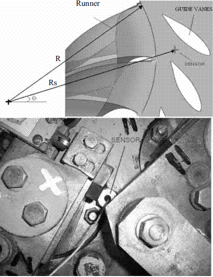
Figure 5 Top: example of sensor location in the stator. Bottom: photograph of the experimental location of the sensor
Moreover, another six dynamic pressure sensors were installed in two transversal sections along the draft tube. The objective of these sensors was to obtain information on the vortex rope generated at the exit of the runner. The two cross sections: i.e. A and B, are shown in figure 6.
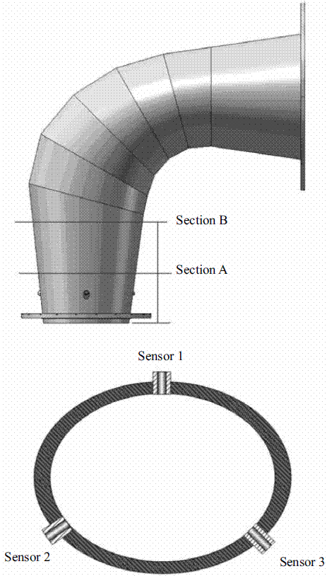
Figure 6 Distribution of the sensors in the draft tube
The measurements were recorded with a simultaneous sampling, with a duration of 3 seconds for every channel at 102 kHz, i.e. more than 40 rotor revolutions and more than 6500 samples per channel. This configuration allowed to capture the hydraulic phenomena present at low and high frequencies.
For the measurement of the torque, a strain gage technique applied to the generation shaft was used. The use of this technique do not interfere with the normal running of the turbine. The strain gage signals were registered via wireless connection into the computer station. For the measurement of the radial force it was use of 4 bi-axial weldable strain gages meanwhile the measurement of the torque used 1 bi-axial weldable strain gage. The strain gages were connected to a transmitter tied to the shaft.
The experimental information given by all this pressure sensors and the strain gages, along different operation points, was used to validate the CFD numerical model, reproducing the same scenarios and operating conditions.
Results
Hill chart results
Prediction of the hill chart consists of, by means of numerical simulations, obtaining the dimensionless values of φ and  needed to build up the characteristic curves under different operating conditions.
The discharge coefficient is the volumetric flow dimensionless number  where Q is the volumetric flow, w the rotation velocity and R the runner radius, whereas the dimensionless energy coefficient is given by
  withE the specific hydraulic energy between the runner inlet and outlet. This energy is calculated by integrating the available hydraulic energy (kinetic plus potential) along the corresponding surface. E is then essentially the mechanical energy transferred by the fluid to the runner.
To numerically determine the hill chart of a Francis Turbine it is necessary to perform simulations for different opening percentages and considering different volumetric flows for each opening. For instance, for an opening of 72.55% five simulations were run with volumetric flows of 4.8, 2.7, 2.0, 1.6 and 1.2 m3/s. The same volumetric flows were considered for the openings of 43.88%, 36.76%, 27.86% and 24.91%. This means 25 simulations, for the same head of 230 m, which corresponds to the real turbine operating conditions.
Figure 7 (top) shows the numerical hill chart obtained. The x-axis represents a normalized value of the discharge coefficient respect the value of φ calculated for the opening of 72.55% and a volumetric flow of 4.8 m3/s, φ*. The y-axis represents the energy coefficient normalized regarding the mentioned value of , *. Each curve is for a different opening percentage, which are shown in the upper part of the figure. A similar behaviour for each opening can be inferred in the different volumetric flows employed. As the opening decreases, the curve tends to grow faster, which is the expected result for Francis turbines. The bottom part of figure 7 represents the normalised efficiency for each opening and different volume flows. It can be clearly seen that for each opening percentage a maximum efficiency exists for a determined volume flow.
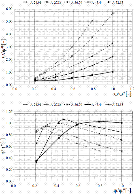
Figure 7 Hill charts of the considered Francis turbine. Top: specific energy. Bottom: efficiency. All values are made nondimensional with the values corresponding to the nominal operating point
Figure 8 presents a comparison between the numerical and experimental results for the curves of torque-volume flow (top) and power-volume flow (bottom) of the turbine. In can be readily observed that for optimum loading the accuracy of the CFD predictions is very satisfactory, and even for moderately partial loads or low volume flow, the CFD results are close to the measurements.
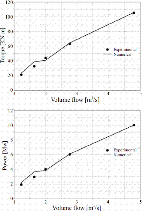
Figure 8 Comparison of numerical and experimental results for the considered turbine. Torque versus volume flow (top) and power versus volume flow (bottom)
Rotor-stator interaction results
The unsteady numerical simulations allowed to calculate the temporal variation of pressure in any point as well as the torque and radial force for the runner blades. Using the utilities of the ANSYS CFX-Post® software, it was generated a spatial point with the same coordinates as the dynamic pressure sensor in the turbine, allowing a direct comparison of the numerical and experimental results. However, the pressure sensors measure only changes in the pressure value whereas the numerical simulation provides the absolute pressure values. Therefore, both data were made dimensionless with the pressure coefficient [11], defined as:
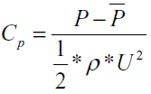
where CP = pressure coefficient [-], P = local pressure,  = mean pressure in the considered interval, ρ = density and U = runner tangential velocity.
The measurement data of pressure were led to the frequency domain in order to investigate the unsteady hydraulic phenomena such as the vortex rope and the rotor-stator interaction, which appear in different components at determined frequencies. However, as it has been said previously, in this paper the attention is focused on the rotor-stator interaction.
Figure 9, top, presents the pressure fluctuations phase averaged, represented by means of the pressure coefficient Cp versus time for the nominal operating point of the machine. Each time series lasts 0.07 s, which equals the time needed by the runner to rotate 1 turn under nominal operating conditions. The experimental signal is the solid line and the numerical the discontinuous line. It can be seen that there is a good agreement between both signals, although there is small discrepancies in the amplitude (less than 5%).
Both signals were transformed to the frequency domain, which is shown in the bottom part of figure 9. In such plot, it can be readily distinguished the frequency of 225 Hz, which represents the characteristic frequency of the expected rotor-stator interaction of the turbine. This result is accurately reproduced by the numerical simulations, which illustrates the ability of numerical simulations for describing satisfactorily the unsteady phenomena in Francis turbines.
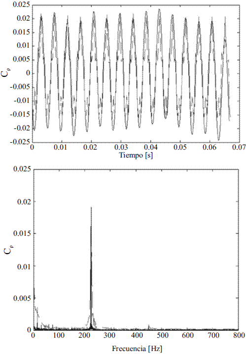
Figure 9 Fluctuating pressure signal in the time domain (top) and in the frequency domain (bottom) for the nominal operating point of the turbine. Experiments: solid line; Numerical results: discontinuous line
Conclusions
This paper shows the utility of the numerical simulations as a tool for design and optimization of hydraulic turbines. The first part has presented the proper methodology to follow in performing the numerical simulations, which depends on the type of phenomena sought, steady or unsteady. Particularly, it has been performed the numerical simulation of the flow inside a Francis turbine currently operating in Colombia. The numerical results agree very well with the experimental measurements for both, the hill chart (steady simulation) and the rotor-stator interaction -(unsteady simulation).
Acknowledgements
The support received from the EAFIT University, EPM, EPFL - LMH Laussane (Switzerland), the Alberta University (Canada), the Universidad Autónoma de Occidente and Colciencias is gratefully acknowledged.
References
1. T. Iwase, K. Sugimura, R. Shimada. Technique for designing forward curved blades fans using CFD and numerical optimization. Proc. FEDSM2006, 2006 ASME Joint U.S. - European Fluids Engineering Summer Meeting. July 17-20 Miami (FL) USA. 2006. Paper FEDSM2006-98136. [ Links ]
2. J. Wu, K. Shimmei, K. Tani, K. Niikura, J. Sato. CFD - based design optimization for hydro turbines. ASME J. Fluids Eng. Vol. 129. 2007. pp. 159-168. [ Links ]
3. H. Keck, M. Sick. Thirty years of numerical flow simulation in hydraulic turbomachines. Acta Mechanica. Vol. 201. 2008. pp. 211-229. [ Links ]
4. Z. Qian, J. Yang, W. Huai. Numerical simulation and analysis of pressure pulsation in Francis hydraulic turbine with air admission. J. Hydrodynamics. Vol. 19. 2007. pp. 467-472. [ Links ]
5. T. C. Vu, W. Shyy. Performance prediction by viscous flow analysis for Francis turbine runners. ASME J. Fluids Eng. Vol 116. 1994. pp. 116-120. [ Links ]
6. M. Sabourin, Y. Labrecque, V. Henau. From components to complete turbine numerical simulation. Proc. of 18th Symp. on Hydraulic Machinery and Cavitation. Valencia (Spain). 1996. pp. 248-256. [ Links ]
7. A. Ruprecht, M. Heitele, T. Helmrich, P Faigle, W. Morser. Numerical modelling of unsteady flow in a Francis turbine. Proc. XIX IAHR Symp. on Hydraulic Machinery and Cavitation. Singapore. 1998. pp. 202- 209. [ Links ]
8. A. Ruprecht, M. Heitele, T. Helmrich, W. Moser, T. Aschenbrenner. Numerical simulation of a complete Francis turbine including unsteady rotorestator interaction. Proc. 20th IAHR Symposium on Hydraulic Machinery and Systems. Charlotte. August 2000. pp. 1-8. [ Links ]
9. F. R. Menter. Zonal Two Equation k-ω Turbulence Models for Aerodynamic Flows. AIAA 1994. Paper 93-2906.- [ Links ]
10. T. C. Vu, B. Nenneman, G. D. Ciocan, M. S. Iliescu, O. Braun, F. Avellan. Experimental Study and Unsteady Simulation of the FLINDT Draft Tube Rotating Vortex Rope. Proceedings of the Hydro 2004 Conference. Porto. Portugal. 2004. pp. 1-12. [ Links ]
11. A. Zobeiri, J. L. Kueny, M. Farhat, F. Avellan. Pump turbine rotor-stator interactions in generating mode: pressure fluctuations in distributor channel. Proc. 23th IAHR symposium.Yokohama. Japan. 2006. pp. 1-10. [ Links ]
(Recibido el 20 de febrero de 2009. Aceptado el 24 de agosto de 2009)
*Autor de correspondencia: teléfono: + 57 +2 + 318 80 00, fax + 57 +2 + 555 44 75, correo electrónico: slain@uao.edu.co (S. Laín).

