A harmony search algorithm for clustering with feature selection

Un algoritmo de búsqueda armónica para clustering con selección de características

Carlos Cobos ^{1,2 *}, Elizabeth León², Martha Mendoza¹

¹ Information Technology Research Group (GTI), Electronic and Telecommunications Engineering Faculty, University of Cauca, Sector Tulcán Office 422 FIET, Popayán, Colombia.

² Research Laboratory of Intelligent Systems (LISI), National University of Colombia, Bogotá, Colombia.

 

---

Abstract

This paper presents a new clustering algorithm, called IHSK, with feature selection in a linear order of complexity. The algorithm is based on the combination of the harmony search and K-means algorithms. Feature selection uses both the concept of variability and a heuristic method that penalizes the presence of dimensions with a low probability of contributing to the current solution. The algorithm was tested with sets of synthetic and real data, obtaining promising results.

Keywords: harmony search, clustering, feature selection

---

Resumen:

En este artículo se presenta un nuevo algoritmo de clustering denominado IHSK, con la capacidad de seleccionar características en un orden de complejidad lineal. El algoritmo es inspirado en la combinación de los algoritmos de búsqueda armónica y K-means. Para la selección de las características se usó el concepto de variabilidad y un método heurístico que penaliza la presencia de dimensiones con baja probabilidad de aportar en la solución actual. El algoritmo fue probado con conjuntos de datos sintéticos y reales, obteniendo resultados prometedores.

palabras clave: búsqueda armónica, agrupamiento, selección de características

---

Introduction

Clustering is the process of partitioning a set of objects into an a priori unknown number of clusters (or groups) while minimizing the within- cluster variability and maximizing the between cluster variability. Clustering is a challenging task in unsupervised learning. It has been used in many engineering and scientific disciplines such as computer vision (e.g. image segmentation), information retrieval (clustering web documents), biology (clustering of genome data) and market research (market segmentation and data forecasting). Several general clustering algorithm categories or approaches have been proposed in the literature, including: hierarchical, partitional, density-based and grid-based algorithms [1, 2]. Partitional clustering has long been the most popular, because it is dynamic, has good performance and it considers the global shape and size of clusters. In partitional clustering, each data object is represented by a vector of features. The algorithm organizes the objects into K clusters in such a way that the total deviation of each cluster is minimized and the clusters centers are far away from each other. The deviation between two points can be computed separately using similarity or distance functions. Most partitional algorithms (e.g. K-means, k-medoids) assume all features to be equally important for clustering, but this approach can create some difficulties because in reality some features may be redundant, others may be irrelevant, and some can even mislead the clustering process. Feature Selection (FS) is the task of selecting the best feature subset in a high- dimensional data set [3]. FS is a very important task in clustering, because it can improve the performance of the clustering algorithm and can contribute to the interpretability of the models generated. FS is usually done before the clustering process in algorithms commonly referred to as filters, but recently, there have been some algorithms (called wrappers) that combine FS simultaneously with the clustering process [3]. In this paper, we have put forward a new partitional algorithm for clustering with FS called IHSK. This algorithm is based on the harmony search (HS) [4­6] and K-means algorithms. HS is used as a global approach to optimize solutions of K-means (best local solutions) in which FS based on variance analysis is done.

Harmony search algorithm

HS is a meta-heuristic algorithm mimicking the improvisation process of musicians (where music players improvise the pitches of their instruments to obtain better harmony) [4-6]. HS has been successfully applied to many optimization problems (e.g. travelling salesman problem, chaotic systems). The steps in the procedure of HS are as follows [4-6]:

1. Initialize the Problem and Algorithm Parameters: The optimization problem is defined as minimize (or maximize) f (x) subject to x_i e X, i = 1,2..., N, where f (x) is the objective function, x is the set of each decision variable x_i, N is the number of decision variables, X_i is the set of the possible range of values for each decision variable, that is , _Lx_i ≤X_I ≤ Ux_i and Lx_i and Ux_i are the lower and upper bounds for each decision variable. In addition, the parameters of the HS are specified in this step. These parameters are the Harmony Memory Size (HMS, a typical value is between 4 and 10), Harmony Memory Considering Rate (HMCR, a typical value is 0.95), Pitch Adjusting Rate (PAR, a typical value is between 0.3 and 0.99), distance BandWidth (BW, the amount of change for pitch adjustments) and the Number of Improvisations (NI) or stopping criterion [4-6].


2. Initialize the Harmony Memory: The Harmony Memory (HM) is a memory location where all the solution vectors (sets of decision variables) are stored. The initial HS is generated from a uniform distribution in the ranges _Lx_i and Uxi, where 1≤ i ≤ N. This step is carried out as follows: x_i ^j =_Lx_t + Randx (_Ux_i - _Lx_i), where j = 1,2... HMS; and Rand is a uniformly distributed random number between 0 and 1 (Rand ~ U(0,1).

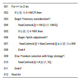
1. Improvise a New Harmony: Generating a new harmony is called improvisation. A new harmony vector, x^T = (x₁ ^T, x₂ ^T , . . .     x^T_N), is generated based on three rules: memory consideration, pitch adjustment and random selection. In this step, HM consideration, pitch adjustment or random selection is applied to each variable of the New Harmony vector in turn.
2. Update the Harmony Memory: The New Harmony vector, xT = (x1 T, x2 T , . . .     xTN) replaces the worst harmony vector in the HM, if its fitness (judged in terms of the objective function value) is better than the second one. The New Harmony vector is included in the HM and the existing worst harmony vector is excluded from the HM.
3. Check the Stopping Criterion: If the stopping criterion (e.g. maximum NI) is satisfied, computation is terminated. Otherwise, Steps 3 and 4 are repeated.

The HMCR and PAR parameters of the HS help the method in searching for globally and locally improved solutions, respectively. PAR and BW have a profound effect on the performance of the HS algorithm. Thus, fine tuning these two parameters is very important. From these two parameters, BW is more difficult to tune because it can take any value from (0, <x>).

The K-Means clustering algorithm

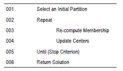
The K-means is a partitioning clustering algorithm. The K-means algorithm is the simplest and most commonly used algorithm employing a Sum of Squared Error (SSE) criterion. This algorithm is popular because it finds a local minimum (or maximum) in a search space, it is easy to implement, and its time complexity is O(n), where n is the number of objects (registers or patterns). Unfortunately, the quality of the result is dependent on the initial points and may converge to a local minimum of the criterion function value if the initial partition is not properly chosen [1,2]. K-means inputs are: The number of clusters (K value) and a set (table, array or collection) containing n objects (or registers) in a D-dimensionality feature space, formality defined by X = {x₁, x₂,...,x_n} (In our case, x_i is a row vector, for implementation reasons). K-means outputs are a set containing K centers. The steps in the procedure of K-means can be summarized as shown in Table 1.

Table 1 The K-means algorithm

Select An Initial Partition: Arbitrarily choose K centers as the initial solution (for example Forgy suggested selecting these K instances randomly from the data set [7]). These K centers are defined as C = {c₁, c₂,... c_k}, and each c_j is an D-dimensionailty row vector.
Re-compute Membership: For all objects in a data set it is necessary to recompute membership according to the current solution. Several similarity or distance measurements can be used. In this work, we used Euclidian distance formality defined as (1).

Each object is assigned to a specific cluster. This assignment is hard or soft. In our case, the assignment is hard, which is defined by Pi,j equal to 1 if x_i e c_j  otherwise is equal to 0.
Update Centers: For some/all clusters in the current solution it is necessary to update centers according to new memberships of the objects. Normally, the cluster center is the mean (average) point (formula 2) of all objects in the cluster, where n. is the number of objects in cluster j.

Until (Stop Criterion): stop if for example, there is no (or minimal) reassignment of patterns to new cluster centers, or there is a minimal decrease in a SSE. The criterion mostly used to distinguish the convergence and to characterize good clusters is based on (3).

Return Solution: return K actual centers C = {c₁, c₂... c_k}.
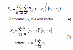
In the literature, various criteria have been used to compare two or more solutions to decide which one is better [8, 9]. The most popular criteria are based on the within-cluster (Sw defined by 4) and between-cluster (S_b defined by 5) scatter matrices. One criteria is the Tmce (S_w^-lS_b). Hence, large values of the criterion correspond to high-quality clustering solutions. This criterion is invariant under any non-singular linear transformation [3] and has been widely used for clustering, where issues such as FS and the number of clusters do not arise.

To calculate S it is necessary to calculate the covariance matrix of features selected. When the variance of a feature is zero or near to zero, that feature is removed from the space of solutions.

Iterative harmony search K-means algorithm with feature selection

Our algorithm, called Iterative Harmony Search K-means Algorithm (IHSK) uses the HS algorithm as a global search strategy across the whole solution space, and the K-means algorithm as a local strategy for improving solutions. In IHSK, each solution vector used in the HS algorithm has different features, and the objective function of the HS algorithm depends on the location of the centroids in each vector solution and the variability of features selected.

Quantitative index for feature selection

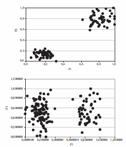
Selecting the relevant features in a clustering problem is a key aspect for improving solutions. From figure 1, we can understand the importance of selecting relevant features. This figure shows a data set with two evident clusters. Feature 1 gives us relevant information to determine two clusters (project data in the F1 and F2 axes), but feature 3 does not (if we project data in the F3 axis, just one cluster appears) so, in this case F3 is an irrelevant feature.

Figure 1 F1 and F2 are relevant features, while F3 is irrelevant

In the literature, FS adopts two kinds of methods [10]: filters and wrappers. Filters preselect the features and then the clustering algorithm works with the selected feature subset. In other words, filters run before and independently from the clustering process [10]. Wrappers involve a clustering algorithm such as K-means, Expectation-Maximization or K-medoids running on a feature subset, with the feature subset being assessed by the clustering algorithm through an appropriate index [3, 10], in our case, the variance of features. Wrappers can offer a better performance, depending on the incorporated clustering algorithm [11].
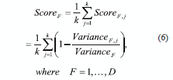
IHSK makes FS an integral part of the global clustering search procedure and attempts to identify high-quality solutions for clustering and FS. Similar to Zeng and Cheung in [12], we determine that a feature is less relevant if the variance of observations in a cluster is closer to the global variance of observations in all clusters. Subsequently, we use the following quantitative index to measure the relevance of each feature:

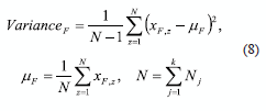
In (6), K is the number of clusters. VarianceFj. is the variance of the j-th cluster projected on the F-th dimension (remember, we are using a data set/table/matrix in a D-dimensionality feature space) and Variance_F is the variance of the F-th dimension.

In (7), Nj is the number of data in the j-th cluster, µ_FJ is the mean (average) of the F-th feature in the j-th cluster, x_Fz correspond to all values in F-th feature of data in the j-th cluster.

In (8), N is the total number of data, mF is the mean (average) of the F-th feature, xFz corresponds to all values in F-th feature.
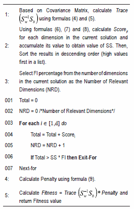
The Score_FJ  indicates the relevance of the F-th feature for the j-th cluster. The Score. indicates the average relevance of the F-th feature to the clustering structure. If Score_F is close to the maximum value, then, all clusters in the current solution are far away from each other on this dimension and hence this feature is very useful for detecting the grouping structure. Otherwise, the Score F will be close to the minimum value. Unlike Zeng and Cheung in [12], we did not use a feature's Markov Blanket to select the appropriate dimensions. We defined a penalty value for the current solution (current selected features) based on the way how Lingo [13] uses the Candidate Label Threshold parameter in the matrix factorization step with Singular Value Decomposition (SVD). Our Heuristic method is based on Score_F values and a new parameter called Percentage of Dimensions (FI). First, we calculate the sum of scores in each dimension, SS       Then, we organize all Score F values (where F = 1,...,d and d < D) in descending order. Next, we iterate and accumulate each ScoreF value until the FI parameter is reached. The number of iterations before reaching the FI parameter is called Number of Relevant Dimensions (NRD). Finally, Penalty for the current solution is equal to (9). For us, when the FI parameter is high (50% or more) we promote lower dimensionality solutions, but if the FI parameter is low, we promote high dimensionality solutions (with 0% the algorithm does not do FS).

Description of Iterative harmony search K-means algorithm

IHSK has a main routine that performs three basic steps. These steps are: initialize the algorithm parameters; initialize the best memory results and call the HSK routine in several iterations; and finally, return the best result. Below, we present these steps in more depth.

1. Initialize the algorithm parameters: in our case, the optimization problem is defined as maximize the product of Trace (S_w^-lS_b) and a
Penalty function (dependent on FSs), called Fitness function. IHSK needs three specific parameters - Best Memory Results Size (BMRS), Number of clusters desired (K), and Percentage of Dimensions (FI) - as well as other parameters from the HS Algorithm (HMS, HMCR, PAR, BW and NI).

2. Initialize the best memory results and call the HSK routine: best memory results (BMR) is a memory location where the best solution vectors are stored. Each row in BMR stores the result of one call to the Harmony Search K-means (HSK) routine, in a basic cycle. Each row vector in BMR has three parts: centroids, a list of dimensions selected and the fitness value of that vector.

 

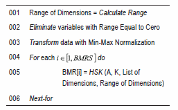
Before starting the process, we calculate the range of each dimension and store these results in a memory location called "Range of Dimensions". Also, we remove decision variables with range equal to zero (0) and transform the data with a Min-Max Normalization [14]. Other tasks of data preprocessing are responsibility of the research person. This step can be summarized as shown in Table 2.
3. Return the best result: find and select the best result from the Best Memory Results (BMR). The best result is the row with the highest fitness value (maximize f (x)). Then return this row as the best clustering solution (centroids, list of dimensions selected and fitness).
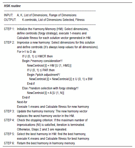
The HSK routine is the HS algorithm with some changes, which works as follows:

• Initialize the Harmony Memory: The HM is a memory location where all the solution vectors are stored. Each vector solution is created with a random number of dimensions (d < D), initial location of centroids (k centroids with Forgy strategy and values in all dimensions) and fitness for this solution. The initial centroids are selected randomly from the original data set (unlike in the original HS algorithm). The general structure of HM is similar to BMR. In this step, we generate HMS vector solutions and then calculate the fitness value for each vector.
• Improvise a New Harmony: A new harmony vector is generated. We use a variation of step 3 in the original HS algorithm to create centroids (each dimension value in each centroid) in the current solution. The random selection process is executed from the original data set (Forgy strategy) (see table 3). Next, we execute one cycle of the K-means algorithm (Algorithm in table 1 steps 3 and 4) and then calculate the fitness value for this solution

Table 2 Initialize the best memory results and call the HSK routine

Table 3 Improvisation of a New Harmony

• Update the Harmony Memory: The New Harmony vector replaces the worst harmony vector in the HM, if its fitness value is better than this latter.
• Check the Stopping criterion: If the maximum number of improvisations (NI) is satisfied, iteration is terminated. Otherwise, Steps 2 and 3 are repeated.
• Select the Best Harmony in HM: We find and select the best harmony, which has the maximum fitness value. Then, we execute the K-means algorithm (Algorithm in Table 1 without step 1, because this solution has information about initial centroids, number of clusters and list of dimensions selected) and then, we calculate a new value of fitness with the final location of centroids.
• Return the Best Result in Harmony Memory: Return the best harmony (centroids, list of dimensions selected and fitness) to IHSK.

To calculate fitness value, we use a function shown in table 4.

Table 4 Routine for calculating fitness value

The HSK routine can be summarized as shown in table 5.

Table 5 Steps in the Harmony Search K-means Routine (HSK)

Complexity

IHSK repeats the HSK routine BMRS times and then carries out a sorting of a vector with BMRS rows. The major computational load occurs in each step of the HSK routine. The HSK routine generates HMS solution vectors and then NI improvisations. For each vector solution generated in the HSK routine, we need to process the variance assessment for FS, Trace (S_w^-1S_b ) calculation and one step of the K-means algorithm. Finally, HSK routine finds and selects the best solution, performs the K-means algorithm for this solution and re-calculates the fitness value (variance and trace). The variance assessment takesO(n *D)times. The Trace (S_w^-1S_b) calculation and one-step of the K-Means algorithm of a given solution take O(n*K*D) and O(n*K*D) times, respectively. The total K-means algorithm and re­calculation of the fitness value take O(n*K*D*L) (where L is the number of iterations taken by the K-means algorithm to converge) times. Therefore, the overall complexity of the proposed algorithm is 0{n*K*D*(L + HMS+ Nl)* BMRS}

Experimental

Data sets

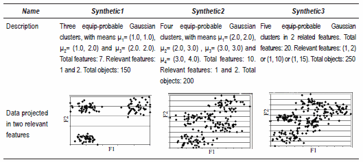
Several data sets (three synthetic and three real), have been used in our experiments. The synthetic data sets were generated with different numbers of clusters and noise. The synthetic data sets contain "relevant" and "irrelevant" features. "Irrelevant" features are generated as Gaussian normal random variables. Table 6 shows the description of synthetic data sets.

Table 6 Description of synthetic data used in our experiments

Three real data sets were considered, they are: Iris, the Wisconsin diagnostic breast cancer (WDBC), and image segmentation. They are taken from the UCI Machine Learning Repository. Table 7 shows the description of real data sets. Since we are concerned with unsupervised learning, the class labels in these data sets are used only for evaluation of the clustering results.

Table 7 Description of real data used in our experiments

IHSK parameters and measures

All parameter values were equal for all data sets. BRMS equal to 10, HMS equal to 25, HMCR equal to 0.95, PAR equal to 0.35, BW equal to 0.0005 and NI equal to 500. K value in each data set was fixed to 3, 4, 5, 3, 2 and 7 respectively. FI was set to 0.3 in the first experiments, and then FI was changed.
In our experiments, we try to solve the following questions: Is the number of clusters correctly identified? and Is the selected feature subset relevant? To answer the first question, we compute Error Classification Percentage (ECP), since we know the "true" clusters or labels of the synthetic and the real data sets. To answer the second question, we use Recall and Precision concepts from the information retrieval field research [14]. In our case, the feature recall (FR) and feature precision (FP) are reported on synthetic data, since the relevant features are known a priori. FR is the number of relevant features in the selected subset divided by the total number of relevant features and FP is the number of relevant features in the selected subset divided by the total number of features selected. High values of FR and FP are desired. This second question cannot be answered for real data because the relevant features are unknown; in this case, we show only the Number of Features Selected (NFS).

Results

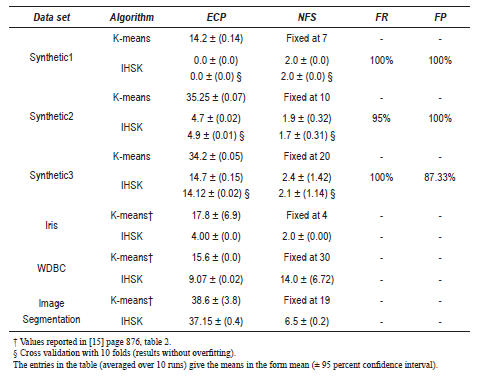
First we conducted a set of experiments on both synthetic and real data to evaluate the proposed algorithm, comparing this with the standard K-means algorithm. We ran the algorithm 10 times and calculated the average to show them as results; these promising results are shown in table 8. IHSK has better results of ECP for both real and synthetic data sets. IHSK is effective in trying to select the relevant features because the results of the NFS are good in synthetics data. Also, FR is higher or equal to 95% and FP is higher than 87%. For synthetic data sets, the K-means algorithm was executed for all features and for the relevant features (K-means-F), but IHSK presented better results.

Table 8 ECP, NFS, Feature Recall (FR) and Feature Precision (FP) by the algorithms

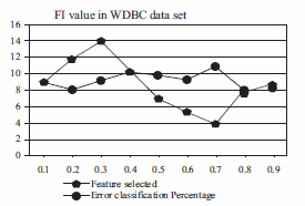
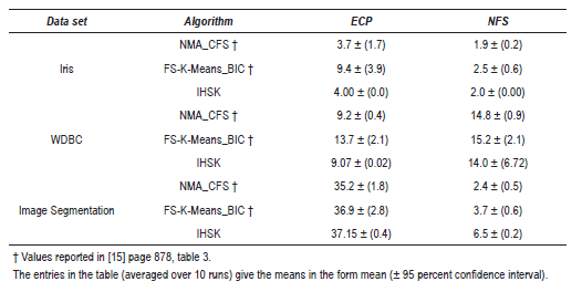
Next, we analyze the FI parameter using the WDBC data set. We ran IHSK with FI equal to 0.1, 0.2, 0.3, 0.4, 0.5, 0.6, 0.7, 0.8 and 0.9. Figure 2 shows the NFS (dash line with triangles) and ECP (line with dots) in IHSK with the different values of FI. In this figure, we can see that if the FI parameter is high we promote lower dimensionality solutions, but if the FI parameter is low, we promote high dimensionality solutions. We can also see that for the WDBC data set, the best solution is with FI equal to 0.8, because the ECP is 7.98% and the NFS is 7.7. We cannot say that high values of FI parameter promise better solutions, because it depends on the characteristics of the data set or the particular application. This analysis is very important in a supervised learning problem, because IHSK can significantly reduce the feature space of the solution. Finally, we compared the results with two new algorithms (see table 9): A niching memetic algorithm for simultaneous clustering and feature selection (called NMA_CFS) and an algorithm for feature selection wrapped around the K-Means algorithm (called FS-K-Means_BIC), both of them proposed in [15]. These two algorithms do FS and find the number of clusters, so results are not totally comparable, but it is nevertheless a good way of fixing a goal for IHSK in a new version. The goal is close to current results in all data sets, but it is necessary to consider including a noise removal procedure in IHSK or use other metrics to compare different cluster solutions with different features selected [3].

Figure 2 ECP and NFS by IHSK with different values of FI parameter

Table 9 ECP and NFS by the three algorithms

Conclusions and future work

We have designed and implemented the IHSK algorithm. IHSK is a wrapper clustering algorithm with a random search strategy, but IHSK can also be used in classification tasks. The improvement of HS and the K-means algorithm with a feature selection process shows promising experimental results. The combination of feature variance, FI parameter and Trace (S_w^-1S_b) shows a new way to find relevant features in a clustering problem with a random strategy search. The overall complexity of IHSK is 0(n*K*D*(L + HMS+ Nl)*BMRS), so IHSK can be used with large data sets. Unfortunately, as with the K-means algorithm, IHSK is sensitive to noise.

There are several tasks for future work; among them: apply the IHSK algorithm to real data sets with a lot of irrelevant and redundant features; include in IHSK a metric (e.g. Bayesian Information Criterion [1]) to find the number of clusters automatically; use the global-best harmony search [5] strategy or other improvements of HS; use K-medoids or Expectation Maximization algorithms instead of the K-means algorithm and compares their results; make IHSK less sensitive to noise; compare IHSK with other initialization techniques of K-means and finally, use another metric for feature selection (e.g. Trace (s_w^-1S_b) normalized using a cross projection scheme [3]).

Acknowledgments

The work in this paper was supported by a Research Grant from the University of Cauca under Project VRI-2560 and the National University of Colombia. We are especially grateful to Guillermo Arenas and Colin McLachlan for their help in reviewing the English text.

References

1. A. K. Jain, M. N. Murty, P. J. Flynn. "Data clustering: a review". ACMComput. Surv. Vol. 31. 1999. pp. 264323.         [ Links ]

2. K. Jacob, N. Charles, T. Marc. Grouping Multidimensional Data Recent Advances in Clustering. Ed. Springer-Verlag. New York. 2006. pp. 25-72.         [ Links ]

3. J. Dy, G.C.E. Brodley, J. Mach. "Feature Selection for Unsupervised Learning". Learn. Res. Vol.5. 2004. pp. 845-889.         [ Links ]

4. Z. Geem, J. Kim, G.V. Loganathan. "A New Heuristic Optimization Algorithm". Harmony Search Simulation. Vol.76. 2001. pp. 60-68.         [ Links ]

5. M. G. H Omran, M. Mahdavi. "Global-best harmony search". Applied Mathematics and Computation, Vol. 198. 2008. pp. 643-656.         [ Links ]

6. M. Mahdavi, M. Fesanghary, E. Damangir. "An improved harmony search algorithm for solving optimization problems". Applied Mathematics and Computation. Vol. 188. 2007. pp. 1567-1579.         [ Links ]

7. S. J. Redmondand, C. Heneghan. "A method for initialising the K-means clustering algorithm using kd- trees". Pattern Recognition Letters. Vol. 28. 2007. pp. 965-973.         [ Links ]

8. A. K Jain, R.C. Dubes. Algorithms for clustering data. Ed. Prentice-Hall Inc. Englewood Cliffs (NJ.). 1988. pp.143-222.         [ Links ]

9. A. Webb. Statistical Pattern Recognition. 2a ed. Ed. John Wiley & Sons. Malvern (UK) 2002. pp. 361408.         [ Links ]

10. A. L. Blum, P. Langley. "Selection of relevant features and examples in machine learning". Artificial Intelligence. Vol. 97. 1997. pp. 245-271.         [ Links ]

11. K. Ron, H. J. George. "Wrappers for feature subset selection". Artif. Intell. Vol. 97. 1997. pp. 273-324.         [ Links ]

12. H. Zeng, Y. M. Cheung. "A new feature selection method for Gaussian mixture clustering". Pattern Recognition. Vol. 42. 2009. pp. 243-250.         [ Links ]

13. S. Osinski, J. Stefanowski, D. Weiss. "Lingo search results clustering algorithm based on Singular Value Decomposition". International Conference on Intelligent Information Systems (IIPWM). Zakapore (Poland). 2004. pp. 359-397.         [ Links ]

14. J. Han, M. Kamber. Data Mining Concepts and Techniques. 2a ed. Ed.Morgan Kaufmann Publishers. 2006.pp.71-72.         [ Links ]

15. S. Weiguo, L. Xiaohui, M. Fairhurst. "A Niching Memetic Algorithm for Simultaneous Clustering and Feature Selection". IEEE Transactions on Knowledge and Data Engineering. Vol. 20. 2008. pp. 868-879.         [ Links ]

 

(Recibido el 29 de Abril de 2009. Aceptado el 6 de abril de 2010)

^*Autor de correspondencia: teléfono: + 57 + 2 + 820 98 00 ext. 2119, fax: + 57 + 2 + 820 98 00 ext. 2102, correo electrónico: ccobos@ unicauca.edu.co. (C. Cobos)