Semantic assessment of similarity between raster elevation datasets

Valoración semántica de la similitud entre conjuntos de datos raster de elevación

Marco Moreno-Ibarra^* , Miguel Torres, Rolando Quintero, Giovanni Guzman, Rolando Menchaca-Mendez

Centro de Investigación en Computación - Instituto Politécnico Nacional Av. Juan de Dios Bátiz S/N, UPALM, C.P. 07738, Mexico, D. F. Mexico.

---

Abstract

This paper describes a method to assess the similarity between digital elevation models (DEM), based on the comparison of the landforms. The method attempts to mimic the one commonly used by human beings, which consists of comparisons among the shapes that a human subject identifies in the landscape. To do so, semantic similarity measurements are applied over a hierarchy of concepts. Our method is composed of two stages: the Geomorphometric Analysis and the Semantic Analysis. The first stage aims to represent the topographic properties using one of the concepts of the hierarchy, depending on an analysis of the DEM. The second stage consists of comparisons among the concepts that characterize the landscape using a measure of semantic similarity. In this stage, two levels of semantic analysis are defined: local and global. The advantage of our method is that the interpretation of the results is simplified by means of a semantic processing.

Keywords:Semantic similarity, DEM, ontology, geomorphometric analysis, GIS.

---

Resumen

Este artículo describe un método para evaluar la similitud entre modelos digitales de elevación (DEM) con base en la comparación de las formas del terreno. El método intenta imitar la forma en que el ser humano compara el paisaje, identificando las formas del relieve. Para ello, se aplican mediciones de similitud semántica sobre una jerarquía de conceptos. El método se compone de dos etapas: Análisis Geomorfométrico y Análisis Semántico. La primera consiste en representar las formas del terreno utilizando alguno de los conceptos de la jerarquía, en función del análisis al DEM. La segunda consiste en comparar los conceptos que caracterizan el relieve, utilizando una medida de similitud semántica. En esta etapa se definen dos niveles de análisis: local y global. La ventaja del método es facilitar la interpretación de los resultados, a través del procesamiento semántico.

Palabras clave: similitud semántica, MDE, ontología, análisis geomorfométrico, SIG.

---

Introduction

Nowadays, it is common to find diverse representations of the same geographic phenomenon [1]. This is mainly due to the development of technologies such as geopositioning, remote sensing and to the fact that geographic data are acquired with different goals and from different perspectives [1, 2]. Hence, it is common for designers and users of the Geographic Information Systems (GIS) to come across data that is the representation of a geographic domain from diverse points of view [2, 3]. One of the most relevant aspects to geographic analysis is the land's topography, which is directly related to natural and social processes [4]. The topography is commonly represented by means of DEMs where the precision of the elevations and resolution are taken into consideration [5]. However, for particular applications, the landforms are the most relevant aspects to be considered, so as to describe if it is steep or flat. The topographical characteristics are intuitively used by the designers to assess if a DEM fulfills the requirements of an application. In this paper we propose a comparative method for DEMs based on semantic similarity between the landform concepts represented in a hierarchy that describes the landscape. This is different from previous works, which are in general oriented towards the analysis and comparison of elevation data based on numerical approaches (e.g., [6, 7]). We propose to use the Terrain Ruggedness Index (TRI) [8] to characterize the topography. The TRI refers to how rugged or irregular is the Earth's surface in a particular area. A semantic approach is used in this paper to analyze the data in a similar way to the one used by a person who interprets qualitative variables [9]. Other approach to semantically process geomorphometric objects is presented in [10, 11]. That is why a hierarchy of landform concepts describes the semantics of the domain of interest. Within the context of this document a concept is an idea, which characterizes a set or category of objects [12]. In our case, it refers to the landforms presented by a portion of DEM. The above is done when transforming quantitative measurements into a concept level with the goal of facilitating its characterization and interpretation. The comparison is based on semantic similarity between the concepts. In general, semantic similarity refers to how similar two concepts are [13], according to their conceptual structure. For example, a mountain is similar to a hill, but they are not exactly the same due to the fact that some of their properties and relations are different (e.g., elevation, size and slope).

Semantic similarity has been used in the past with diverse objectives, such as: information retrieval [14] and generalization of geographic data [9]. However, to the best of our knowledge there is no previous work related to the comparison of DEMs based on semantic similarity. As a case study, our method is applied to two geographic datasets of Mexico.

The rest of this paper is organized as follows: the related work is presented in the Background section. Then, we describe the proposed methodology, as well as the experiments and results. Finally, we outline our general conclusions.

Background

A brief state ofthe art about ruggedness measuring of topography is included as well as some terms and concepts related to how we measure the semantic similarity.

Methodology

Measurements of terrain ruggedness

Our method is based on geomorphometric analysis that is defined as the measuring of the geometry of the Earth, using raster data to analyze the distribution and concentration of spatial objects [15]. Some methods have been defined to quantify ruggedness [16], where it corresponds to the total length of the elevation contours, presented in a particular area. Other methods are based on the density of the contour lines per unit of area [17].

The TRI [8] is based on qualitative descriptors to characterize DEMs in such a way that the derived values are easily understood. The method to compute the TRI consists of two stages: (a) the elevation analysis, the elevations are directly analyzed from the model, having as a result a quantitative descriptor; while (b) the tagged stage generates the quantitative descriptors, by the usage of the previously defined intervals. The stage (a) consists of calculating the differences between the elevation values, starting from a central cell within an 8-neighborhood. Later on, the differences of elevation among the 8-neighbors of each cell are squared so as to make an arithmetic addition of the squares of all the differences of elevation. The quantitative descriptor of the TRI is the result of the calculation of the square root of the addition, and it corresponds to the mean elevation of the change between any point of the DEM and the area, which surrounds it. Thus, the units of the result will be given in meters. Equation 1 demonstrates the described procedure.

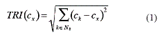
where: c_x is the cell under analysis and N₈(c) is the set of 8-neighbors of c.

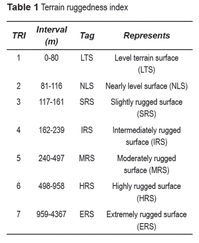
The stage (b) consists of classifying the quantitative values according to the intervals proposed by [8]. A tag is assigned to each cell in relation to the classification to which it belongs to (see table 1). However, they can be modified to highlight certain aspects of the topography, depending on the specific case study.

Semantic Similarity

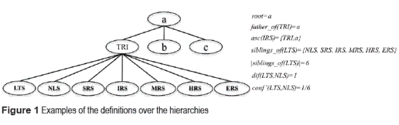
Semantic similarity allows the identification of objects, which are conceptually close to each other but not identical [13]. We focus on the evaluation of the conceptual distances, also called confusion that was redefined in this work, and which is applied over hierarchies [18]. Some terms related to confusion and hierarchies are defined (see figure 1) as follows:

• Hierarchy. A hierarchy is a 2-tuple H(C_H , R_H) where C_H is a set of concepts and R_H is a set of relations of the form aρb, where a,b ∈ C_H and ρ is a relation ρ: C_H x C_H, of the form aρc, aρb ∈ R_H then, b = c a ∈ C_H.

• Additionally, a_iρb = U(b) where U(b) is the universe of elements that can be identified by b.

• Ordered Hierarchy, H is an ordered hierarchy if b ∈ C_H , Ω: U(b) x U(b) such that Ω is a relation of order.

• Father of, let a, b ∈ C_H be concepts, then father_of (a) = b, iff aρb ∈ R_H.

• Son of, let a, b ∈ C_H be concepts, then son_of = b, iff aρa ∈ R_H, on the other hand son_ of (b) = {a| aρb ∈ R_H}.

• Root, is the node h which does not have father, that is h ∈ C_H | father_of (h) = Ø.

• Siblings, let a, b ∈ C_H be two concepts. Then, they are siblings if father_of (a) = fathers_of (b). The set of the siblings of a concept a is defined as siblings_of (a) = sons_of (father_ of (a))-{a}.

• Ascendants, the set of ascendants of a concept a ∈ C_H is defined by asc(a) = {b} asc (b), where b = father_of (a).

• Difference between concepts in a ordered hierarchy, this function is only defined over sibling concepts. It is defined as dif (a, b) = ω(b) - ω(a), where ω is a function that computes the position of a concept in an order Ω. More formally, ω(a) = |{c_i|c_iΩa}, ω(b) = |{c_i|c_iΩb}. Additionally, dif (a,b) = 0 ↔ a = b.

• Confusion in simple hierarchies. To measure confusion, the descendant links are counted from r to s. If r,s ∈ C_H, then the confusion of using r instead of s, denoted as conf(r,s), is defined by the following rules:
conf(r,r) = conf(r, asc(r)) = 0.
conf(r,s) = 1 + conf(r, father_ of(s)).

• Confusion in ordered hierarchies. For simple hierarchies composed of ordered sets, the confusion of using r instead of s, denoted by conf'(r,s), is defined by:
conf' (r,r) = conf (r, asc (r)) = 0.
If r and s are siblings and the father is not in an ordered set; then, conf'(r,s) is the relative distance from r to s, being the number of steps required to get from r to s in the order defined by Ω, divided between son_of(r)) - 1.
conf(r,r)' = 1 + conf'(r, father_of (s)).

Semantic comparison of digital elevation models (SECODEM)

The SECODEM method is based on measuring of semantic similarity over a hierarchy of geomorphometric concepts. The procedure is carried out taking into account a base dataset (CB) and a secondary dataset (CS). Preferably, the one that owns the highest level of detail, or the most accurate is considered as CB. However, the selection can also be random. SECODEM consists of two stages: Geomorphometric Analysis and Semantic Analysis. In the first stage, the numerical analysis of the DEM is carried out. The objective is to assign to each cell of the DEM a quantitative descriptor representing its ruggedness. The latter is done by an integer value defined in the TRI column of table 1. This task is performed for the CB as well as for the CS. The Semantic Analysis stage compares the DEMs by means of a measure denominated confusion, which represents the conceptual distance between concepts that describes the ruggedness in CS and CB. This measure is used because we are conceptualizing the domain through a hierarchy. From this, two levels of semantic analysis are generated: local and global.

Stage 1: Geomorphometric analysis

This stage extracts the topographic properties implicitly represented in the DEM. TRI is used to characterize DEMs, identifying the most relevant aspects of each region. The values retrieved from the set are denoted by: TRI = {LTS, NLS, SRS, IRS, MRS, HRS, ERS}, which describe an explicit meaning of a landform (see table 1). Still, other classifications of the topography can be made, like the one defined by [19], which considers aspects such as slope and curvature. Figure 2 depicts the pseudo code of the TRI algorithm.

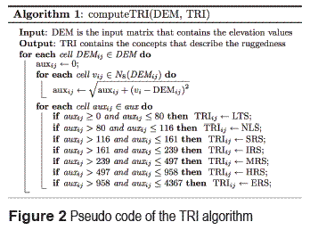
In the previous pseudo code, DEM is the input matrix that contains the elevation values, DEM_ij is the value of the matrix DEM that corresponds to the elevation at that coordinate in the i,j position. The aux matrix stores the quantitative descriptors that characterize the ruggedness. These descriptors are later classified using the ruggedness intervals established in [8] and presented in table 1. By using this method, we are able to qualitatively quantify the ruggedness and hence, interpret them as concepts in the hierarchy. The classified values are stored in a raster called TRI that contains the concepts that describe the ruggedness.

Stage 2: Semantic analysis

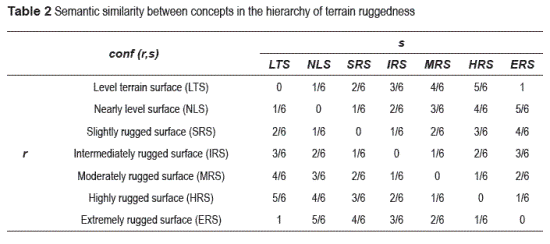
In this stage a comparison between the descriptors in the DEM that refer to the two datasets to be compared (CB and CS) is performed. Such comparison is attained in a concept level, by means of a measure of the semantic similarity; which is commonly defined in terms of a distance between two concepts. These concepts belong to a hierarchical structure, which underlies in an ontology [9, 13]. In this case, an ordered hierarchy based on the ruggedness describing the concepts related to the TRI (see table 1) is used. That is, the concept, which represents the highest ruggedness, will appear in one extreme of the hierarchy partition whereas the concept, which represents the lowest ruggedness, will appear in the opposite extreme. These values are preceded by their cardinality. The hierarchy of concepts of the TRI was implemented in the Ontology Editor Protégé 3.4.1. We are using only the relation of existence ("is") to define the concepts that belong to the same classification, allowing it to be specialized by means of generic concepts that explicitly describe the concept terms defined in [8]. The comparison is done in two levels: local and global.

Semantic similarity in a local level

The semantic similarity in a local level is defined in terms of the functions defined over the hierarchies presented in the Semantic Similarity Section. This similarity is established between two concepts that describe the TRIs and is computed as the difference between them within the hierarchy, divided by their total number of siblings (see equation 2).

Please note, that if the TRIs are the same then the numerator will be zero. In this case, the confusion in a local level will be zero. On the other hand, the denominator cannot take a value of zero because hierarchies are complete partitions composed of at least two parts. Therefore, if a is one of the parts, then the minimum value that the expression siblings_of(a) can take is one (see equation 2).

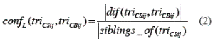
where, tri_CSij and tri_CBij refer to a cell of the raster with values of TRI for CS and CB, respectively. In fact, the similarity is evaluated considering the absolute value of the difference of the positions of two concepts that appear in the hierarchy. The possible values of the similarity are in the interval [0, 1], (see table 2). In this table is appreciated that the more similar two concepts are, the less their value of similarity will be.

If other geomorphometric measurement is applied, like the classification in [19], another kind of structure will be required, and in some cases, another measure of semantic similarity, as the one described in [13] will be also required. Based on the measures concerning hierarchy, two cases of semantic similarity (i.e., equivalent and different) are defined to a local level among the cells belonging to two DEMs. In this case, confusion and a threshold value (w) are used. This threshold is defined by the user according to the requirements of the case study. The cases of semantic similarity in a local level are:

- Equivalent, if 0 < conf_L(r,s) < w <1, the concepts are defined as equivalent, which means that the topography being compared may be considered as the same.

- Different, if 0 < w < conf_L(r,s) < 1 , the concepts are considered different. Thisinterpretation is because the topographical characteristics are diverse.

Semantic similarity in a global level

This measurement uses the semantic similarity at a local level, defined in equation 3.

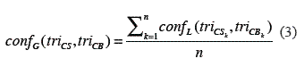
where, tri_CS and tri_CB are the rasters that store the TRI of each dataset and n is the number of cells that contains tri_CS and tri_CB. The range of this function is between 0 and 1. Values near conf_G = 0 mean high similarity or equivalence between DEMs, while values near conf_G = 1 are interpreted as DEMs that are not similar. Furthermore, the global measurement allows the introduction of new concepts to characterize qualitatively the differences between the CS and CB of the DEMs. These concepts are:

- Identical, if conf_G = 0; means that landforms in CS are identical to CB, and CS can be considered equal to CB.

- Substitute, if 0 < conf_G ≤ 0.04; means that CS can be substituted by CB.

- Very similar, if 0.04 < conf_G ≤ 0.12; means that CS and CB have a large number of landforms in common.

- Similar, if 0.12 < conf_G ≤ 0.25; means that CS and CB have several landforms in common.

- Somehow similar , if 0.25 < conf_G ≤ 0.46; means that CS and CB have some landforms in common.

- Different, if 0.47 < conf_G ≤ 1; means that CS and CB have just a few or any landforms in common.

The intervals to determine the semantic similarity in this level, were established by experimentation, using the consensus of geologists, as is presented in [9]. However, the intervals can be calibrated depending on the application.

Considerations of implementation

The following considerations have been established taking into account that the comparison is achieved at a conceptual level. It is important to point out that in our methodology the rasters have to refer exactly to the same geographic area. Thus:

- DEMs must have the same coordinates system, projection, datum and units.

- DEMs must have the same geometric resolution.

- If the bounding coordinates of the DEMs are different, the comparison must be made only with the overlapping cells.

Ideally the semantic processing avoids the usage of the aspects that traditionally are used for the manipulation of digital cartography such as scales and geographic coordinates.

Results and discussion

In this section, a set of results when applying the method to the DEMs of Mexico is presented. They were generated from elevation contour lines from INEGI (National Mapping Agency of Mexico) that correspond to two different editions of the topographic map E14A56 to a scale of 1:50,000. The contour lines are given by intervals of elevation of 10 m, being the minor elevation equal to 950 amsl and the major elevation equal to 2200 amsl. DEMs with resolution of 50 m, having 263 rows and 399 columns were generated (see table 3). The resolution was determined based on the surface that covers the area and in such a way that the topography of the terrain, which is not considerably large.

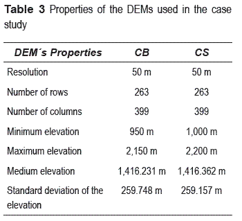
Figure 3.a shows the DEM that represents the CB, while figure 3.b depicts the CS. In these figures it is appreciated that both models are very similar; however, they are not the same. The TRI computation allows the characterization of the topography and it is applied to quantify the similarity between the DEMs. Figure 3.c shows the TRI for the CB, where the minimum value of the TRI is identified as 1 (Level terrain surface), while the maximum value is 7 (Extremely rugged surface), (see table 1) and the average value is 3.919. This can be interpreted (approximating it to the nearest integer number) as a zone, which is mainly "Intermediately rugged surface" (IRS). In figure 3.d, the TRI for CS is shown, the minimum value of TRI is 1, while the maximum TRI is 7.

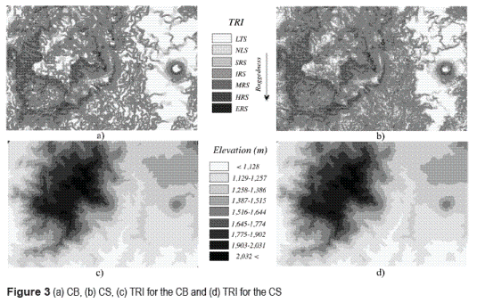
Therefore, the medium value is 4.212, which can be interpreted as a zone that in general is an IRS. In both cases, it can be noticed that the zones identified as extremely rugged are located in the western part of the area, while the flat zones are located mainly in the east section of the DEM.

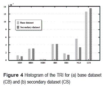
When analyzing the histogram for the TRI for the CB (figure 4.a) and the one for the TRI for the CS (figure 4.b), it is observed that in both cases the most popular class is a flat surface identified by the concept "Level terrain surface" (SPL) (see table 1). However, it is important to notice that in the rest of the classes, do not have the same degree of popularity. In general, it can be assumed that the datasets are similar.

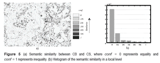
As a consequence, a measure of semantic similarity at a local level is applied, which will allow us to semantically quantify the differences between the DEMs. The semantic similarity between the raster that holds the TRI for the CB and the one that holds the TRI for the CS is shown in figure 5.a. When visually analyzing figure 5.a, it can be intuitively said that both datasets are similar; this is due to the fact that the light tones in such figure are predominant. Note that in the figure the light tones indicate similarity between datasets, in other words the values of similarity are close to zero. In particular, large zones with values of similarity equal to zero located to the western part of the area can be appreciated. This means that the same landform is described in both datasets, while in the whole area; there are also zones where considerable differences in the topography conf = 1 can be appreciated. Such statement is confirmed when observing the histogram of figure 5.b, where the most popular class is conf = 0. The latter means that the landforms are the same. Likewise, it is depicted in the histogram that the cardinality of the classes decreases with respect to the difference between concepts. In these experiments, the cases of semantic similarity at local level were identified as "equivalent" and "different", using a threshold value of w = 1/6. In this case, the number of elements that belong to the equivalent class is larger than the number of elements that belong to the different class (see figure 5.a). This can be appreciated when observing figure 5.b. By using the concepts of "equivalent" and "different", the semantic similarity is described at a local level. With the purpose of quantifying the semantic similarity at a global level, the measure conf_G is applied, which is 0.089 for this case. Taking into account the previously defined criterion, it can be said that the datasets are very similar. This corresponds to the interpretation given in figure 5.a.

Conclusions

In this work, a method based on semantic similarity to compare DEMs, using the geomorphologic characteristics has been described. The method is based on a hierarchical representation of the concepts and properties, in particular the Terrain Ruggedness Index. A semantic component is added to the data, which is usually not considered in the traditional quantitative approaches used in GIS. The goal is to extract the semantics of the elevation dataset by means of a geomorphometric analysis. This process provides as result, an evaluation based on the meaning of these representations, where we take advantage of an explicit, precise and comprehensible vocabulary denoted by concepts that makes easy the interpretation of the results. To describe the semantic similarity between the DEMs, two levels of analysis are proposed: local and global. The first one describes the semantics of a single cell and the latter describes the semantics of whole DEM. The assessment and comparison of the elevation data have an important role in diverse areas of application such as prevention of natural disasters, agricultural planning, and hydrology, in which the correct selection of the data determines the success of any kind of spatial analysis.

Acknowledgements

Work partially sponsored by the IPN, by the CONACyT under grant 106692 and by the SIP-IPN under grants 20101282, 20101069, 20101088, 20100371, and 20100417. We are thankful to the reviewers for their invaluable and constructive feedback that helped improve the quality of the paper.

References

1. D. Sheeren, S. Mustiére, J. D. Zucker. "A data- mining approach for assessing consistency between multiple representations in spatial databases". Int. J. of Geographical Information Science. Vol. 23. 2009. pp. 961- 992.         [ Links ]

2. P. Fisher, A. Comber, R. Wadsworth. "What's in a name? Semantics, standards and data quality". R. Devillers, H. Goodchild. (editors). Spatial data quality. From process to decisions. Ed. CRC Press. Boca Raton. 2010. pp. 2-16.

3. H. T. Uitermark, P. J. van Oosterom, N. J. I. Mars, M. Molenaar. "Ontology-based integration of topographic data sets". Int. J. of Applied Earth Observation and Geoinformation. Vol. 7. 2005. pp. 97-106.         [ Links ]

4. J. M. Sappington, K. M. Longshore. "Quantifying Landscape Ruggedness for Animal Habitat Analysis: A Case Study Using Bighorn Sheep in the Mojave Desert". J. of Wildlife Management. Vol. 71. 2007. pp. 1419-1426.         [ Links ]

5. O. Z. Chaudhry, W. A. Mackaness. "Creating Mountains out of Mole Hills: Automatic Identification of Hills and Ranges Using Morphometric Analysis". Transactions in GIS. Vol. 12. 2008. pp. 567-589.         [ Links ]

6. E. R. Venteris, B. K. Slater. "A Comparison between Contour Elevation Data Sources for DEM Creation and Soil Carbon Prediction, Coshocton, Ohio". Transactions in GIS. Vol. 9. 2005. pp. 179-198.         [ Links ]

7. S. Clarke, K. Burnett. "Comparison of Digital Elevation Models for Aquatic Data Development". Photogrammetric Engineering & Remote Sensing. Vol. 69. 2003. pp. 1367-1375.         [ Links ]

8. S. J. Riley, S. D. De Gloria, R. Elliot. "A terrain ruggedness index that quantifies topographic heterogeneity". Intermountain J. of Sciences. Vol. 5. 1999. pp. 23-27.         [ Links ]

9. M. Moreno-Ibarra. "Semantic Similarity Applied to Generalization of Geospatial Data". Lecture Notes in Computer Science. Vol. 4853. 2007. pp. 247-255.         [ Links ]

10. R. Quintero. Representación Semántica de Datos Espaciales Raster. Tesis Doctoral. Instituto Politécnico Nacional. 2007. pp. 77-108.         [ Links ]

11. R. Quintero, M. Torres, M. Moreno, G. Guzmán G. "Metodología para generar una Representación Semántica de Datos Raster". T. Delgado, J. Capote (editors). Semántica espacial y descubrimiento de conocimiento para desarrollo sostenible. Ed. CUJAE. La Habana. 2009. pp. 119-145.         [ Links ]

12. S. A. Sloman, B. C. Love, A. Woo-Kyoung. "Feature centrality and conceptual coherence". Cognitive Science. Vol. 22. 1998. pp. 189-228.         [ Links ]

13. A. Rodriguez, M. Egenhofer. "Comparing Geospatial Entity Classes: An Asymmetric and Context- Dependent Similarity Measure". Int. Journal of Geographical Information Science. Vol. 18. 2004. pp. 229-256.         [ Links ]

14. K. Janowicz, C. Keßler, M. Schwarz, M. Wilkes, I. Panov, M. Espeter, B. Bäumer. "Algorithm, Implementation and Application of the SIM-DL Similarity Server". Lecture Notes in Computer Science. Vol. 4853. 2007. pp. 128-145.         [ Links ]

15. R. Bonk. "Scale-dependent Geomorphometric Analysis for Glacier Mapping at Nanga Parbat: GRASS GIS Approach". Proc. of the Open source GIS - GRASS User's Conference. Trento (Italy). 11-13 september 2002.         [ Links ]

16. S. L. Beasom, E. P. Wiggers R. J. Giordono. "A technique for assessing land surface ruggedness". J. of Wildlife Management. Vol. 47. 1983. pp. 1163-1166.         [ Links ]

17. J. S. Jenness. "Calculating landscape surface area from digital elevation models". Wildlife Society Bulletin. Vol. 32. 2004. pp. 829-839.         [ Links ]

18. S. Levachkine, A. Guzman-Arenas. "Hierarchy as a new data type for qualitative variables". Expert Systems with Applications. Vol. 32. 2007. pp. 899-910.         [ Links ]

19. D. J. Pennock, B. J. Zebarth, E. de Jong. "Landform classification and soil distribution in hummocky terrain, Sasketchewan, Canada". Geoderma. Vol. 40. 1997. pp. 297-315.         [ Links ]

(Recibido el 13 de agostoo de 2010. Aceptado el 21 de febrero de 2011)

^*Autor de correspondencia: teléfono: + 52 + 55 + 57 29 60 00 ext. 56528, fax: + 52 + 55 + 57 29 6000 ext. 56607, correo electrónico: marcomoreno@cic.ipn.mx. . (M. Moreno-Ibarra)