Tactical planning of domestic supply chains

Planificación táctica de las cadenas de abastecimiento domésticas

Rafael Guillermo García-Cáceres*¹, Fernando Palacios-Gómez², Mario Ernesto Martínez-Avella³

¹Department of Industrial Engineering. Escuela Colombiana de Ingeniería. Autopista Norte Ak 45 N.° 205-59. Bloque C 2do Piso. Bogotá, Colombia.

²Calle 119 N.° 72B-60, Apto 104. Bogotá, Colombia.

³Postgraduate Institute - FORUM. Universidad de la Sabana. Cra. 69 N.° 80-45, of. 301 Bogotá, Colombia.

---

Abstract

This paper presents a single-period mathematical programming model NLMIP of a 5-stage supply chain with multiple possibilities of organizational ownership that allows several distribution channel links. The objective of the model is to optimize profit after tax, taking into account transfer prices, economies of scale, agreements between agents, demand and inventory issues, among other relevant aspects, specially in an idealised domestic environments. Finally, a solution procedure is presented for the problem associated with the NLMIP mathematical programming model proposed, that gives an optimal solution in satisfactory computational time. The model was validated using an experiment based on computational simulations.

Keywords: Supply chain management, integer programming, non-linear programming, logistics.

---

Resumen

Este artículo presenta un modelo de programación matemática NLMIP de un periodo simple para una cadena de abastecimiento de 5 etapas con múltiples posibilidades organizacionales de propiedad en los canales de distribución. El objetivo del modelo es optimizar la utilidad después de impuestos, contemplando entre otras consideraciones, precios de transferencia, economías de escala, acuerdos entre agentes, demanda, inventario, en un ambientedoméstico de decisión. Finalmente, presenta un procedimiento de solución del NLMIP que proporciona soluciones óptimas en tiempos razonables. El modelo fue validado por medio de un experimento computacional.

Palabras clave: Administración de la cadena de abastecimiento, programación NLMIP, logística.

---

Introduction

Recent progress made in supply chains has been focused on global environments. It emerged as the logical consequence of initial developments in domestic environments. However, in spite of the significant progress made in global environments, a great part of this background has not been transferred to domestic environments, and additionally many important aspects have been ignored or have not been considered simultaneously for decision making. Consequently, the aim of this paper is to incorporate several considerations omitted or not incorporated in the tactical and domestic supply chain bibliography into one single idealised model.

To achieve this goal, a review of work on tactical supply chain decision-making is presented, which describes relevant aspects for both modelling and solution procedures. The work presented here aims to establish a model that takes into account some considerations identified in the literature review that are relevant for domestic environments. A mathematical programming model non linear mix integer (NLMIP) is presented, along with a solution procedure that intends to satisfy such needs.

Backgroud

The following review is focused on the description of some topics considered relevant on tactical decision making in domestic supply chains and that have been treated by means of mathematical programming models.

One first review was developed by [1]. The author makes a description of the relevant aspects on supply chain modeling of single echelon systems with deterministic demand. The fundamental tactical aspects were associated with distribution of raw materials and final products. The size of the problems was limited by the absence of a computationally adequate MIP optimizer. The evolution of the investigation in tactical supply chains has been developed in several ways. On the one hand, as was indicated by the author, towards dynamic modeling considerations and handling of inventories associated with an one member of a specific echelon within the supply chain (agent) [2]. On the other hand there was an increasing tendency towards a greater satisfaction of the final consumer [3], to consider developments of information and communication systems since the end of the nineties and eighties [4], the information structure [5], and later towards better coordination of the logistics operations between the different stages of the supply chain, procurement, production and distribution [6].The aspects considered were: lead times, capacities of the procurement and distribution channels, economies of scale, bill of materials, among others. Towards the end of the twentieth century the increased pressure by the economic internationalization, and new developments in computational processing created global supply chain [7], new aspects had to be considered these included: demand uncertain considerations, transfer prices, taxes and duties, exchange rates, among others, but not the modelling of alliances. Solutions were developed incorporating solution procedures supported in commercial software [8] that resulted in satisfactory practical results [7].Others topics related with our study, include procurement uncertainty in the demand for products [9, 10], and transfer prices [11, 12].

Supply chain considerations

The pertinent literature allows to development of multi-stage supply chains has been limited to the context of a physical network where the distribution is organized by distribution centers (DC) [4]. However, although this is quite common in global environments, it can not be found in most practical cases in domestic environments, where plants can for instance, supply demand zones (DZ) directly. It is common in the literature, to find considerations with respect to the capacity in strategic rather than tactical contexts. Nevertheless, the problem of capacity in tactical decision-making is important, and it is associated with the handling of throughput of product families. Finally, the simultaneous explicit inclusion of transfer prices (TP) and economies of scale (SE) in supply chain models is conspicuous through absence in the literature. On the other hand, mathematical programming modelling in the supply chain context has been limited to problems having few logistics echelons [13]. Due to their combinatorial nature the treatment of supply chains has been limited to relate to production inside plants, without taking into account that transformation processes can be carried out in sales points associated with DZs (afifth stage not considered in the current literature). On the other hand, when a company has integratedDZs, the possibility of surplus, or demand deficit should also be considered, due to the demand variability.

In conclusion, except for some qualitative conditions that may exist in specified supply chains situations, that require application of Integral Analysis Method -IAM- [14], we aim to include those aspects that are considered most relevant to making tactical decisions, particularly in domestic environments. Within this context, a proposed model and solution process can be used as a reference for future studies.

Economies of scale and expandablecapacities

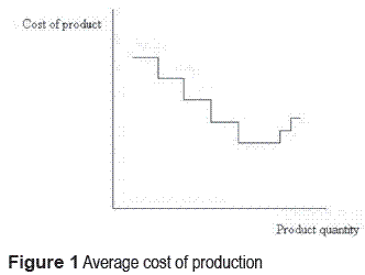
The typical behaviour of SE is represented by the function shown in figure 1, where the averagacost decreases up to a point where production capacity is fully used, and increases again when that capacity is exceeded and subcontracting or the use of stocks become necessary to satisfy demand. SE can be achieved through technological, organizational and pecuniary factors [15, 16].

Transfer pricing

A TP is the price that a selling department, division or subsidiary of a company charges for a product or service supplied to a buying department, division, or subsidiary of the same firm [17]. As proposed in this paper the approach suggested by [11] is used as a basis for this model.

Distribution

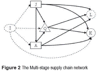
Figure 2 shows a network with a wide range of possibilities for distribution and various forms of ownership organization in the domestic supply chain. Dotted lines represent subcontracted suppliers already established in the market, while continuous lines represent agents who are vertically integrated or are associated through alliances. In order to facilitate the reading of the article, we will denominate with the word "integrated" those business units that are owned by the organization or associated with it through alliances. A global possibility that can be modeled in a domestic context is offered by INCOTERM "Delivery Duty Paid" (DDP).

Where: I = External suppliers. J = Integrated plants that supply goods to subsidiary plants. A = Integrated plants that do not supply goods to subsidiaiyplants.Q = Integrated distribution centers (DC). K = Integrated demand zones (DZ). L = Non integrated demand zones (DZ).

Finally, one single distribution channel managed by the salesperson was assumed, since this is the condition most frequently found in domestic environments.

Demand

The model is based on the assumption that it is possible to satisfy the demand for goods in non-integrated DZs. In the case of integrated DZs, surplus or deficit associated with the demand is allowed, with the purpose of finding an optimum balance in production based on the estimation of average demand.

Storage

The proposal made by [18] is used to handle inventories transferred between agents and inventories transferred from DCs to integrated DZs. It includes considerations about safe stocks, security cycle factors, trip frequency, and inventory cycles, and assumes that the demand and the lead time of an item are independent of each other. This approach is particularly effective for practical matters.

Capacity

The model includes constraints on throughput capacity for each associated stock family in each one of the stages of the supply chain, since this is the condition usually found in real cases.

Bill of materials

The model includes constraints on bills of materials (BOM) for each facility where a transformation activity takes place, and for each raw material or input used in that activity. This condition is more explicit than the usual single constraint set. In the case of DCs, a unique mass balance set constraint is caused by each case, because no transformation processes take place in them.

Model

The associated model (P1) is show below:

Indices and Sets:

In addition to the sets presented to illustrate the supply chain network in figure 2, the following are included:

D: Nodes of supply chain network

E: Operation scales. E(_*,b): Operation scales of item b supplied by facility type *,where* Є D.

F: Item families. F(_*): Item families of facility type *,where* Є D. F(▫,▪): Item families transported between the facility ▫ and the facility type ▪,where(▫, ▪) Є N.

M:  Handled products and input material. M(q): Items handled by DC q. M(_*,q): Items handled by DC q and supplied by supplier *, where* Є D.

N : Arcs of supply chain network.

P: Products. P(_*): Products supplied by supplier *, where* Є D. P(▫,▪): Products of the facility ▫ supplied by the facility type ▪,where(▫, ▪) Є N. P(k,b1): Goods produced in integrated DZ k that use item b1 as input

R: Raw materials or input. R(_*): Raw materials used by facility type *, where* Є D. R(▫,▪): Raw materials of facility type ▪ supplied by supplier ▫,(▫, ▪) Є N.

▪(▫): Facility type ▪ supplied by the facility type ▫,where (▫, ▪) Є N. ▫(▪): Facility type ▫ who supplies facility type ▪,where(▫, ▪) Є N. ▫(▪,b1): Facilities type ▫ which supplies facility type ▪ with item b1,where ▫ Є D. ▫(▪,b) : Facility type ▫ supplied by facility type ▪ with item b, where (▫, ▪) Є N.

In order to facilitar the read of paper the parameters are denoted with xx and the variables with xx, they are presented in each constraint group.

Objective Function: Maximize: Profit after tax

Where: uα_*⁺=  Net income before tax of facility type * in the time period, where * Є D. uα_*^-=  Loss before tax of facility type * in the time period, where * Є D. IR_*= Tax on facility type * in the planning period ($ / plant), where * Є D.

Constraints:

Pre-tax net income in each facility

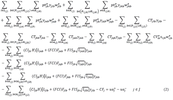
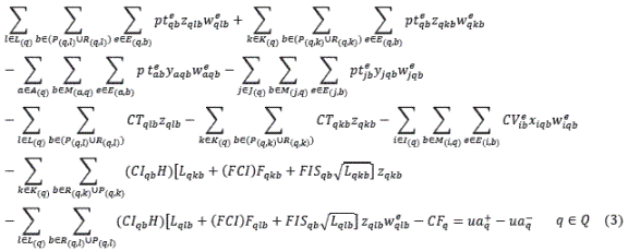
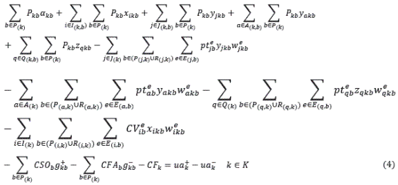
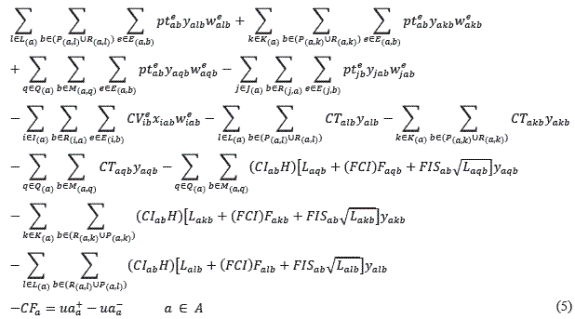
Parameters: FCI = Inventory cycle factor (percentage). FIS_*b =Security stock factor for item b in facility type * (Item units / Planning period), where ▫ Є D. F_▫▪b= Frequency of trips between facility type ▫ and facility type ▪ for item b  (Time units / Planning period), where(▫, ▪) ЄN. H = Fraction of inventory keeping in one period. Holding cost given in $/($. units of time) (units of time consistent with those of the average transportation time parameters defined below) [in general, given in $/$. year]. L_▫▪b= Lead time taken by facility type ▫ to deliver item b to facility type ▪ (Time units / item), where (▫, ▪) Є N. CF_*= Fixed cost of facility type * in the planning period ($ / planning period), where * Є D. CFA_kb= Cost of deficit for item b in integrated DZ k ($ / item). CI_*b= Inventory cost for item b  in facility type * in the planning period ($ / item). CSO_kb= Cost of surplus of item b in integrated DZ k ($ / item). CT_▫▪b= Initial unit transportation cost of item b from facility type ▫ to facility type ▪ ($ / item), where (▫, ▪) Є N. CV_ib^e= Cost of item b provided by supplier i at operation scale e ($ / item). P_kb= Sale price of item b inDZ k ($ / product unit).

Variables: α_kb= Item b used to satisfy the demand of DZ k in the time period. x_i*b^e= Item b supplied by supplier i to facility type * at scale e per planning period, where * Є D. y_▫▪b^e= Item b supplied by facility type ▫ to facility type ▪ at scale e per planning period, where (▫, ▪) Є N. z_q▪b^e= Item b supplied by the DC q to the DZ ▪ (K, L) at scale e per planning period, where (▫, ▪) Є N.  w_▫▪b^e= binary variable that take a value 1 if the item b from facility type ▫ is supplied by the facility type ▪ in the scale e, where (▫, ▪) Є N, and 0 in otherwise.

The next expression takes into account the pre-tax net income for the complete set of plants that supply integrated plants.

Expression for integrated DC’s net income:

Expression for DZ’s net income:

Expression for the net income of plants receiving products from subsidiary plants:

Expressions for modeling the scale operation of each facility type are modeled by the following type of constraints. In this case for the scale operation of external suppliers:

Where x_i*b = Item b supplied by supplier i to facility type * per planning period,where * Є D.

where: GMAX_ib^e= Maximum supply of item b provided by supplier i at scale e per planning period (Item units / Planning period). GMIN_ib^e= Minimum supply of item b provided by supplier i at scale e per planning period (Item units / Planning period).

An alternative modelling for the scale operation of the external suppliers can be expressed for this case as follows:

BIG = Big positive number. G_ib^e: Oferta de la artículo b suministrado por el proveedor i en la escala e por periodo de planeación (Unidades del artículo / Periodo de planeación).

Demand in integrated DZ:

Where: g_kb⁺=  Surplus of item b in DZ k. g_kb^-=  Deficit of item b in DZ k. pt_*b^e = TP of item b from facility type * in scale e per planning period, where * Є (D). Γ_*b= Demand for item b in DZ type * per planning period (Item units / Planning period), where * Є D.

Demand in non-integrated DZ:

Mass balance at distribution center:

Production and handling capacity per item are modeled by the following type of constraints. In this case for plant supplying subsidiary plants:

T_▫b= Capacity units used by facility type ▫ to produce one unit of item b (Resource units / item). Where ▫ Є D. T_▫▪b= Capacity units used in the transportation of item b between facility type ▫ and facility type ▪ (Resource units / item), where (▫, ▪) Є N. CAPP_*b =Production capacity of plant type * for item b per planning period (Resource units / Planning period), where * Є D.

Bill of materials is modeled by the following type of constraints. In this case for plants supplying subsidiary ones:

where Q_b1b2 = Quantity of item b1 used in the production of item b2 (Volume or weight units of item b1 / item b2)

Item-family inventory capacity is modeled by the following type of constraints. In this case for plants supplying subsidiary ones:

CAPI_*f = Finished-product inventory capacity of family f in facility type * in the planning period (Volume or weight / Planning period), where * Є D. V_fb= Volume or weight of item b in the stock place associated with family f in the planning period (Volume or weight / item)

Transportation capacity is modeled by the following type of constraints. In this case between DC and both integrated and not-integrated DZs:

CAPT_▫▪f = Carrying capacity of the means of transportation associated with family f  that is used between facility type ▫ and facility type ▪ in the planning period (Volume or weight / Planning period), where (▫, ▪) Є N.

Transfer-price bounds are modeled by the following type of constraints. In this case in plants supplying subsidiary ones:

PTMAX_*b^e = Upper bound of TP of item b in facility type * in scale e in the time period, where * Є (D). PTMIN_*b^e = Lower bound of TP of item b in facility type ▫ in scale e in the time period, where * Є D.

Flow bounds are modeled by the following type of constraints. In this case of supplier:

SMAX_*b= Maximum supply of item b agreed by supplier ▫ (Item units / Planning period), where * Є D. SMIN_*b= Minimum supply of item b agreed by supplier * (Item units / Planning period), where * Є D.

The decision variables are nonnegative

Solution process

For solving the problem, three steps are proposed:

Step 1. Redefinition of variables: The non-linear nature of equations 2 to 5 is simplified; the nonlinearity treated arise from the product of the two continuous, non-negative flow variables and the TP associated with them is replaced by a non-negative continuous variable. The method employed is illustrated by equations 23 through 26 (the latter being related to equation 9). The result is an equivalent problem (called P3), which is also a bilinear and non-linear MIP problem but more treatable.

Step 2. Definition of bounds: The vectors of the lower bound (UMIN) and the upper bound (UMAX) arises of pre-tax profit variables for each of the integrated agents involved in the supply chain, and the objective function bounds are calculated. In order to determine bound vectors, the number of scale levels of P3 is reduced to one, TP are fixed to their maximum (minimum) value, and input costs are fixed to their minimum (maximum) value for each flow. Consequently, two versions of the relaxed problem (denominated P2) are obtained. In summarizing, this linear problem allows the calculation of the profit bounds of the original problem (P1). The mathematical programming problem P2 is bilinear. According to [19] it is an NP-hard problem.

Step3. P3 solution: In order to solve P1, a procedure based on the inclusion of additional constraints on P3 is proposed. First, upper and lower bounds of the pre-tax profit vector and of profit objective bounds obtained from the previous step are included. Additionally, from the transformation presented by [20] to approximate the nonlinearity of the problem, new variables are redefined and new constraints are added to previous constraints of P3. Finally, a binary search algorithm is proposed.

Redefinition of variables (in this point is necessary to have as reference the model NLMIP presented above with equations A*)

These are the new non negatives variables:

Alternatively for equation 9

And affect the equations (2 to 5), and the equation (9) as:

Also it affects the constraints associated to the TP. In order to illustrate it, the constraints associated to the bounds of flows that leave the integrated plants that supply goods to subsidiary plants are used (equation 17):

Constraints associated with the previous equations are included. And Alternatively: Equation (8):

Definition of bounds

The two bilinear models, P2, are based on model P1 as follows:

First P2 Model: TP and flow costs are fixed as follows:

Second P2 Model: TP and flow costs are fixed as follows:

Scale summations and their associated binary variables are eliminated in equations 2 to 5, and flows bounds constraints are modified in order to establish flow bounds in the new variables. In order to illustrate it, equation 2 (below) is used:

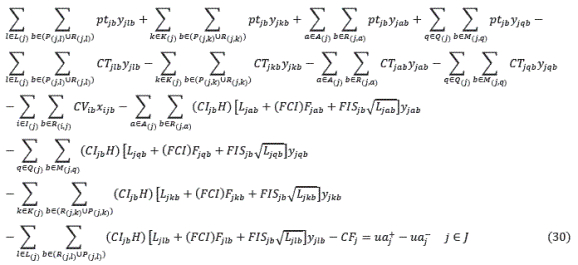
Flow constraints are replaced by the following expressions that establish flow bounds between each echelon of the supply chain, as was mentioned earlier. As an example, the constraints associated with the flows of integrated DCs to integrated DZs are used:

Where G▫▪^emin represents the minimum bound of flow associated with the smaller scale between two echelons, and G▫▪^emax represents the maximum bound of flow associated with the larger scale associated in the original problem (P1). 

Finally, the constraints of TP are eliminated.

The problem P2 is efficiently solved by means of the successive LP solution procedure introduced by Vidal and Goetschalckx [11], and represents a relaxed version of this problem. As was mentioned previously, the solutions for pre-tax profit and objective profit bounds of each business unit and objective solution obtained in this step are used as virtual upper and lower bounds of P3.

P3 solution procedure

In order to solve P3, the bilinear nature of equations 2 to 5 associated with each unit businessare treated by setting pre-tax profits. These values are calculated from the maximum and minimum bounds obtained from P2 as:

Upper bound of pre-tax profits vector, UMAX: Max (U_{FIRST P2}, U_{SECOND P2}).

Lower bound of pre-tax profits vector, UMIN: Min (U_{FIRST P2}, U_{SECOND P2}).

And similarity:

Upper bound of total profit, OFMAX: Max (OF_{FIRST P2}, OF_{SECOND P2})

Lower bound of total profit,OFMIN: Min (OF_{FIRST P2}, OF_{SECOND P2})

Where: U_{FIRST P2}: Pre-tax profits vector solution of first P2. U_{SECOND P2}: Pre-tax profits vector solution of second P2. OF_{FIRST P2}: Objective function of first P2. OF_{SECOND P2}: Objective function of second P2

This solution process implies the inclusion of a set of additional constraints to P3. The set of equations is shown below:

The total profit constraint is shown below:

Finally in order to deal with the nonlinearity of P3, [20] transformation was used, for setting product prices for bundling of products. The authors present an approximation that includes substitution of new variables and constraints that are added to problem. This is shown below:

Suppose the product Ω x Ξ appears in a model, where Ξ is binary {0,1} variable while Ω is nonnegative continuous variable, then:

∆ ≤ Ω

∆ ≤ Ξ M_Ξ

∆ ≥ Ω – (1− Ξ) M_Ω

Where:M_Ω :Upper bound on the value of Ω and M_Ξ :Upper bound on the value of Ω x Ξ

In order to use the [20] approach, first the following non negative variables are redefined. These are the new variables:

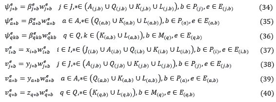
This procedure affects the equations (2 to 5) constraints. In turn to illustrate the previous process, it is presented like example for equation 5:

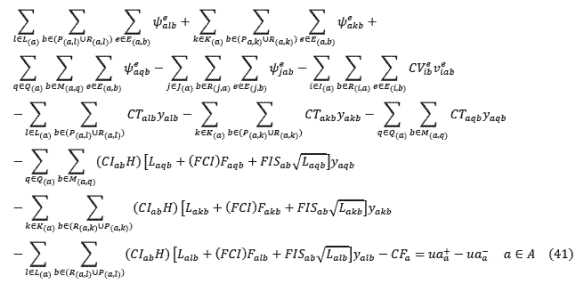
The process also affects the constraints associated with the TP. In order to illustrate the previous assertion, the constraints associated with bounds of the flows that leave the integrated plants that do not supply goods to subsidiary plants, are used:

Constraints associated with the equation ∆ ≤ Ω are included. As an example, the constraints associated with the flow of integrated DCs to integrated DZs are used. Some examples are:

Constraints associated with the equation ∆ ≤ Ξ M_Ξ are included. Some examples are:

Constraints associated with the equation ∆ ≥ Ω –(1− Ξ) M_Ξ are included. In order to illustrate it, some examples are presented:

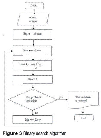
Finally, in order to make the procedure of solution more efficient, the binary search algorithm shown below is used. The above P3 solution process, as already mentioned, leads to the solution of the original problem P1. (see figure 3 )

Computational experience

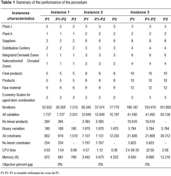
The table 1 below shows the instances of the problem. They are divided in twelve simulated instances of P3 to determine its respective computational complexity. For each instance, their physical and computational characteristics are described in order to analyze its performance (see table 1).

The solution process was supported by MIP commercial software LINGO^TM. In the computations of the instances, Pentium-4 2.8 Ghz, 1 GB RAM and Win XP-SP2 operative system was used. The solutions presented are optimum. The total CPU time is in (min:sec) format.

Conclusions

The most significant contributions of this paper are the design of a mathematical programming model that can be used as a paradigm in the tactical planning of domestic supply chains, and the description of the procedure followed to solve it. An advantage of the solution process proposed is the low significant level of technical expertise required to achieve the fast solution times for the instances studied.

Among the new research possibilities opened up by this paper are the development of new solution procedures (e.g., decomposition methods) that allow the application of the model in larger scales of optimization, and the consideration of qualitative aspects that can be relevant in these types of organizations, such as transaction costs, [14] and so, can be included in the optimization of the supply chain.

Acknowledges

This article is the result of a research project "Optimization of Agro-industrial Chains in Colombia" carried out by La Universidad de la Sabana with financial support of COLCIENCIAS (Colombian Institute for the Development of Science and Technology 'Francisco José de Caldas') and La Universidad de la Sabana, and the scientific collaboration of Escuela Colombiana de Ingeniería Julio Garavito.

References

1. C. H. Aikens. "Facility location models for distribution planning". European Journal of Operational Research. Vol. 22. 1985. pp. 263 - 279.         [ Links ]

2. M. A. Cohen, H. L. Lee. "Strategic analysis of integrated production-distribution systems: Models and methods". Operations Research. Vol. 36. 1988. pp. 216-228.         [ Links ]

3. B. C. Arntzen, G. G. Brintegrated, T. P. Harrison, L. L. Trafton. "Global supply chain management at digital equipment corporation". Interfaces. Vol. 25. 1995. pp. 69-93         [ Links ]

4. A. M. Geoffrion, R. F. Powers. "Twenty years of strategic distribution system design: An evolutionary perspective". Interfaces. Vol. 25. 1995. pp. 105-127.         [ Links ]

5. P. A. Slats, B. Bhola, J. J. M. Evers, G Dijkhuizen. "Logistic chain modeling". European Journal of Operational Research. Vol. 87. 1995. pp. 1-20.         [ Links ]

6. D. Thomas, M. C. Griffin. "Coordinate supply chain management". European Journal of Operational Research. Vol. 94. 1996. pp. 1-15.         [ Links ]

7. C. J. Vidal, M. Goetschalckx. "Strategic production- distribution models: A critical review with emphasis on global supply chain models". European Journal of Operational Research. Vol. 98. 1997. pp. 1-18.         [ Links ]

8. M. Goetschalckx, C. J. Vidal, K. Dogan. "Modeling and design of global logistic system: A review of integrated strategic and tactical models and design algorithms". European Journal of Operational Research. Vol. 143. 2002. pp. 1-18.         [ Links ]

9. A. Gupta, C. D. Maranas. "Managing demand uncertain in supply chain planning". Computers & Chemical Engineering. Vol. 27. 2003. pp. 1219 - 1227.         [ Links ]

10. C. Chen, W. Lee. "Multi-objective optimization of multi-echelon supply chain networks with uncertain product demands and prices". Computers & Chemical Engineering. Vol. 28. 2004. pp. 1131 - 1144.         [ Links ]

11. C. J. Vidal, M. Goetschalckx. "A global supply chain model with transfer pricing and transportation cost allocation". European Journal of Operational Research. Vol. 129. 2001. pp. 134 - 158.         [ Links ]

12. F. Villegas, J. Ouenniche. "A general unconstrained model for transfer pricing in multinational supply chains". European Journal of Operational Research. Vol. 187. 2008. pp. 829 - 856.         [ Links ]

13. G. Mohan. Mixer integer programming models for supply chain integrated planning. Masters Thesis. Concordia University, Montreal. UMI Dissertation Information Service. 2003. pp. 133.         [ Links ]

14. R. G. García, J. A. Araoz. F. Palacios. "Integral Analysis Method - IAM". European Journal of Operational Research. Vol. 192. 2009. pp. 891- 903.         [ Links ]

15. H. Viscencio. Economíapara la Toma de Decisiones. Ed. Paraninfo. México. 2002. pp. 386.         [ Links ]

16. K. C. Tan. "A framework of supply chain management literature". European Journal of Purchasing and Supply Management. Vol. 7. 2001. pp. 39 - 48.         [ Links ]

17. W. M. Abdallah. International Transfer Pricing Policies: Decision Making Guidelines for Multinational Companies. Ed. Quorum Books. New York. 1989. pp. 162.         [ Links ]

18. E. R. Silver, R. Peterson. Decision systems for inventory management and production planning. 2^nd. ed. Ed. Wiley. New York. 1985. pp. 722.         [ Links ]

19. P. M. Pardalos. S. A. Vavasis. "Quadratic programming with one negative eigenvalue is NP-hard." Journal of Global Optimization. Vol. 21. 1991. pp. 843-855.         [ Links ]

20. W. Hanson. R. K. Martin. "Optimal bundle pricing". Management Science. Vol. 36. 1990. pp. 155 - 174.         [ Links ]

(Recibido el 6 de junio de 2009. Aceptado el 10 de mayo de 2011)

^*Autor de correspondencia: teléfono: + 57 + 1 + 668 36 00 ext: 278-279, fax: + 57 + 1 + 676 23 40, correo electrónico: rafael.garcia@escuelaing.edu.co (R. García)