ARTÍCULO ORIGINAL

 

Activity scheduling through gantt charts in an ms excel spreadsheet

 

Diagramas gantt para programación de actividades en el tiempo en diferentes recursos usando ms excel

 

 

Juan P. Caballero Villalobos¹, Sandra P. Jarro Sanabria², Rafael G. García Cáceres^3*

¹Assistant professor and member of CIOL group (Optimization and Logistics Research Center). Department of industrial engineering. Pontificia Universidad Javeriana. Cll 40 No 5–50. Bogotá, Colombia.

²Assistant profesor and director of the Civil Engineering Career at Pontificia Universidad Javeriana. Cll 40 No 5–50 Bogotá, Colombia.

³Associated professor, Co–Director of CIOL group (Optimization and Logistics Research Center), and Director of CIMSER Group (Manufacturing and Services Research Center. Departament of Industrial Engineering. Escuela Colombiana de Ingeniería. A.A. 14520 AK.45 No. 205–59 (Autopista Norte) Bogotá, Colombia.

^*Autor de correspondencia: teléfono: + 57 + 1 + 668 36 00 ext. 278–279, correo electrónico: rafael.garcia@escuelaing.edu.co (R. García)

 

(Recibido el 21 de junio de 2011. Aceptado el 11 de noviembre de 2011)

 

---

Abstract

Effective communication of task–resource assignment plans comprises several challenges in important fields such as production scheduling and/or project management. Said difficulties result from the cost and sophistication level of most project planning information tools, and from the pedagogic challenge implied in getting people with different educational levels to communicate through such tools. The present work introduces the implementation grounds of a simple information technology development for the construction of Gantt charts as decision making support tools for people or companies that have limited access to sophisticated information technology tools. The implementation and execution of the Visual Basic code with Excel applications are described in detail, as well as the correct use of the Excel solver add–in from VBA macros to solve the implemented mathematical models.

Keywords: Directed graphs, Gantt's charts, project management, scheduling, spreadsheet program

---

Resumen

La comunicación efectiva de los planes de asignación de recursos–tareas presenta retos importantes en campos como programación de la producción y/o la gestión de proyectos. Esta dificultad, en parte, se debe al costo y nivel de sofisticación de las herramientas informáticas existentes para la programación de proyectos, y al reto pedagógico que implica su comunicación con personas de disimiles grados de escolaridad. Este trabajo muestra los fundamentos de implementación de un sencillo desarrollo informático para la construcción de diagramas Gantt de uso conveniente para apoyar el desarrollo técnico del proceso de toma de decisiones en compañías o personas que no cuentan con la posibilidad de adquirir sofisticados recursos informáticos. El trabajo describe detalladamente la implementación en Visual Basic para Aplicaciones y adicionalmente muestra el uso del complemento solver de Excel invocado desde macros de VBA para solucionar los modelos matemáticos implementados.

Palabras clave: Grafos dirigidos, diagramas de Gantt, programación de proyectos, programación de la producción, programas en hoja de cálculo

---

 

 

Introduction and background

Gantt charts are project and production management tools (among other possible applications) that allow determining the starting and finishing times of several activities that make use of different resources on a time line. Although described by the author as a graphic development, the original proposal was a table arrangement [1], which not only facilitates an exact comparison of delivered to programmed production quantities, but also allows taking corrective actions. In such doing, it identifies daily production amounts with their corresponding starting and finishing times, which implicitly defines the sequence of operations implied. This type of chart contemplates all the commitments assumed with the client, thus leading to focus attention on overcoming obstacles and preventing delay; and when fulfilling seems impossible, to a timely notification [2]. The importance of Gantt charts has to do with how simple and easy to understand they are, which might be the reason why they have kept their popularity [3]. According to [1], Gantt charts had been identified since the mid 1920's as a useful production planning tool, and even, the original tool that considers the concept of production batch policy without intermediate inventories constituted a first approach to the notion of ''lean production''.

Although the Gantt charts started to be studied since the publication of Taylor's book ''Shop Management'' (1919), they were already in use for controlling daily production since the beginning of the twentieth century [4,5]. Considered for years as the best practice in real production environments, they have evolved with the complexity of production settings, as it is shown by [6,7], among other relevant works.

Even though nowadays one of the most important uses of Gantt charts is their application to project management, it only appeared long after the original proposal had come out. Since then, despite a period of disuse caused by the preponderant utilization of critical path methods, the massive application of Gantt charts as a complementary technique has been increasing lately, to the point of their mandatory inclusion in project management software [8].

From the standpoint of software packages, nowadays there exist several suites for production scheduling and project management that include Gantt charts among their analysis tools [9–11]. Organizations such as APICS, POMS and PMI offer updated information on recent Information Technology advances in the field. Although there is evidence of the development of tailored production scheduling systems in manufacturing and project management companies [3], they are far from being reported at the level of detail of the current one, because they are under intellectual property protection e.g ILOG Inc, Metafuse Inc., and ViewPath Inc, among others.

The present review shows the current relevance of this planning tool, especially in the two cited contexts: production scheduling and project management. Also, it underscores the scarcity of free software resources for building own planning packages by users that cannot afford them. In this sense, this work adheres to [3], who holds that despite their broad applicability to decision making support, Gantt charts are still far from reaching full utilization.

 

Development

Basic concepts

Information technology

Information technology has had a big impact on production scheduling and project management [3]. Regarding our topic, this process has taken three technological ways: 1. Operational research mainly supported on net flow algorithmic and mathematical programming, both embedded in LP [12]. 2. Information technology tools themselves, summarized in computer languages and applications. and 3. Advances in computer processing capacity. Altogether, these three factors have allowed tackling practical problems. In this sense, the present implementation has been set in VBA, counting with an Excel reading– writing interface, and is executable from an ordinary PC; all of which confers it considerable effectuation easiness, as far it has no need of data base experts, low level languages or great execution power.

Said advantage also has to do with the Microsoft Excel solver application, which by using the solver add–in allows solving linear, mixed and non­linear problems whose objectives and constraints can be expressed mathematically. As analogs of the variables of the mathematical model it uses spreadsheet cells to which it assigns the optimal values of the solution of the situation to be worked out. The constraints and the objective function are created through linking formulas between the cells that work as variables and those that contain the parameters of the model.

Basic definitions

Programming is a decision making process that plays an important role in most manufacturing and services companies. It makes use of mathematical techniques or heuristic methods to assign limited resources to the performance of several tasks [13]. In turn, project management implies applying knowledge, abilities, tools and techniques to the execution of a project, in order to achieve its requirements [14]. This institution defines project activities as the elements that are used in fulfilling it. Normally, any activity has an expected duration, cost and resource requirements. Among the latter we can count people, equipments and materials that are necessary to conduct the activity.

The development of the tool is presented below in two sections: the first one describes two strategies for determining the earliest values of the activities, as part of the elaboration of the Gantt diagram. The second section presents the VBA implementation of the strategies treated in the previous section, as well as the corresponding spreadsheet configurations.

Applied Algorithms

Topological order

In an acyclic net G = {N, A}, where N is the set of nodes and A is the set of arcs between pairs of nodes that belong to the net, the latter acquire a topological arrangement if for every (i,j) arc of the net, the topological order assigned to node i is lower than that assigned to nod j [12]. The pseudo–code of a topological order assignment algorithm is presented below:

Topological arrangement algorithm
For every i in N do indegree(i) := 0;
For every (i, j) in A do indegree(j) := indegree(j) + 1;
LIST := ø;
next := 0;
for every i in N do
if indegree( i ) = 0 then LIST := LIST + { i };
while LIST ≠ ø do
Choose a node i from LIST;
LIST := LIST – { i };
next := next + 1;
order(i) := next;
for every (i,j) in A(i) do
indegree( j ) := indegree( j ) – 1;
if indegree( j ) := 0 then LIST := LIST + { j };
end for
end while
if next < n then the graph contains a directed cycle
else the graph is acyclic and has been arranged topologically
end algorithm;

The variable "indegree( j )'', registers, at every moment, how many preceding–j nodes have not been assigned their corresponding topological order in the net. The variable ''next'' counts how many nodes have already been assigned their corresponding topological order in the net.

Label correction algorithms

Frequently used in net flow applications, they are iterative algorithms in which tentative distance labels are assigned, likely to be moved to a new node at every step. These labels only become permanent once the last step of the algorithm has been executed. These algorithms are part of master programs that allow treating more general problems in which an arc representing a negative distance might be found. Also, they can be more flexibly adapted to the problem that needs to be solved. For a review of this concept, we recommend the work of [12].

The pseudo–code of the label correction general algorithm for calculating minimum distances between a dummy node and each of the nodes in a directed non–cyclic net is presented next:

A1 Label correction algorithm
d(s) = 0 and pred(s) = 0;
for every j in N–{s} do d(j) := inf;
as far as any arc (i,j) satisfies
d(j) > d(i) + ci,j do
d(j) := d(i) + cij; pred(j) = i;
end as far as
end algorithm;

The algorithm above allows recalling the minimum distance path that goes from the original node to the other nodes of the net. This is done through the variable pred (j), which traces back the minimum distance path that goes from node j to the original dummy node.

Determination of earliest activity starting times

• Linear Model

This approach assumes that any sequence of activities that makes use of different resources can be expressed by means of a acyclic directed graph. The latter is made up of nodes representing activities, and arcs between nodes, representing precedence relationships between nodes. These arcs have been assigned specific values that represent the time it takes to get to a given activity, starting from the preceding one. Authors such as [12,15,16], among others, present a large series of applications in different fields that make use of this technical approach to define, for example, the precedence relationships that result from the decision to carry out a given activity before another one, with regards to each of the resources needed for such performance.

Several linear models have been associated to this graphic representation. Said models allow finding activity schedules according to different metrics [17]. One of them is particularly adequate for establishing the starting and finishing times of activities, so as to minimize the maximum completion time it takes to execute them all. Below is the mathematical programming formulation used for scheduling the activities of acyclic graph G = {N, A}:

MM1
Sets:
N: Nodes
A: Arcs

Parameters:
p_pi :processing time of activity i
p_ri :release time of activity i

Variables:
v_s_i :starting time of activity i
v_w:maximum completion time

Objective Function:
Minimize z=v_w

Constraints:
v_s_j ≥v_Si +p_p ∀{i,j} A(I)
v_s_i ≥p_r_i ∀i N (II)
v_w≥ v_s_i +p_p_i ∀i N(III)
v_s_i ≥0 ∀i N

The value assigned to variable is the time it takes to start activity i. Variable, as the maximum bound of the completion times of all activities, allows finding the C_max time. It is assumed that no interruption is allowed once the processing of an activity is started.

• Net flow option

This alternative establishes the earliest activity starting times in two stages. The first one assigns the topological order to each node in the acyclic directed graph G = {N, A}. The second one applies the label correction algorithm to estimate the earliest finishing time of each activity, according to their existing precedence relations and release times.

With the aim of eventually counting with activity RELEASE times and not needing the dummy node s proposed by the original label correction algorithm A1, the latter is modified, leading to:

Modified label correction algorithm
for every j in N do d(j) := 0;
scan according to the previously
assigned topological order
if d(i) = 0 then d(i) = r(i) + p(i)
as far as any arc (i,j) satisfies d(j) < d(i) + p(j) do
d(j) := max{ d(i) , r(j) } + p(j);
pred(j) = i;
end as far as
end algorithm;

Where r(i) represents the release time of activity i, and p(i) is the processing time of activity i, which has been assigned lower topological order than activity j.

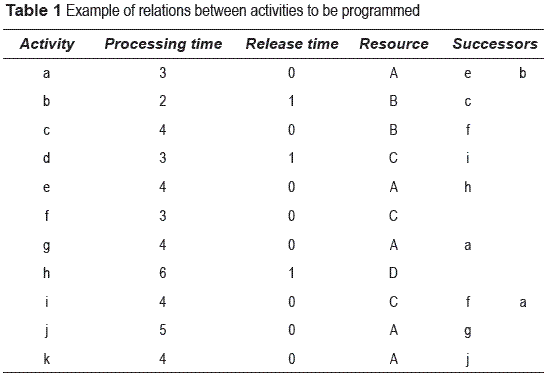
For explanatory purposes, we shall illustrate the following example. Given a problem that seeks to minimize the completion time of its last activity (K), table 1 shows the precedence relations between activities, as well as their completion and technical release times.

.

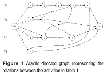
This situation can be represented through the acyclic directed graph shown in figure 1.

In the figure above the solid line arcs represent precedence relations between activities, while the dashed line ones represent existing technical restrictions. The problem presented in table 1 and figure 1 can be solved either by using an lp solver or by the net flow algorithm.

VBA Implementationss

Linear Model

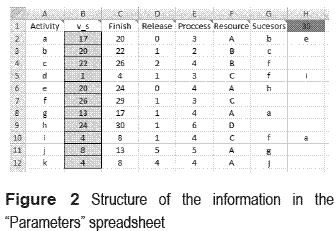
Below is shown the Excel structure designed required to find the parameters used by the algorithms. The structure consists of two spreadsheets. The first one, named Parameters, describes the activities to be programmed, and the existing relationships between them. The first line contains the headings of the columns that, starting from the second line, store homogeneous data, as follows: column A lists the activities of the problem; column B represents the variables; column C expresses the finishing time of the activity, calculated as the sum of its starting values plus its processing time (second and fifth columns, respectively); column D presents the minimal technical time from which the activity can be started (release time); column E contains the completion time of the activity; column F identifies the resource where the activity should be programmed; finally, column G, as well as the following ones, indicate the names of the activities that follow the one in column A. This scheme allows defining multiple precedence relationships between different pairs of activities. Figure 2 presents an example of the Parameters sheet with 11 activities labeled from a to k. The gray cells correspond to the variable v_s associated to each activity; whereas the activities in columns G and the following ones are those that come after the activity in column A.

As a consequence of this arrangement, the interpretation of the information in line 5 of figure 2 goes as follows: the activity identified as d can only be programmed in resource C, starting from time 1, and with a 3 unit processing time. Finally, the existing precedence relations between activities are as follows: d f and d i, implying that neither i nor f can be started before having finished activity d. The Visual Basic code of the linear model is shown below.

1    Solver linear sub model ()
2         Dim a As Object
3         Dim n_activities, line, i, j, successor
4
5         Set a = AddIns(''Solver'')
6         If a.Installed = True Then
7              MsgBox ''The Solver add–in is installed''
8         Else
9              a.Installed = True
10      End If
11
12       'Determine the number of activities to be programmed
13      n_activities = count_n_activities()
14
15       'Resets the solver's default configuration
16       SolverReset
17       SolverOptions Precision:=0.001, AssumeNonNeg:=True, _
18                              AssumeLinear:=True, Iterations:=30000
19
20       'Add max function to the finishing times of the tasks
21       Range(''H1'').Formula = ''=MAX($C$2:$C$'' & n_activities + 1 & '')''
22
23       'Minimize the value of cell "H1" by changing B2 cells to B n_activities+1
24       SolverOK SetCell:=Range("H1"), MaxMinVal:=2, _
25                               ByChange:=Range("B2:B" & n_activities + 1)
26
27       'Addprecedence constraints, relation 3 is > =
28       'Starting times must be greater than, or equal to release times
29       Solveradd cellRef:=''$B$2:$B$'' & n_activities + 1, relation:=3, _
30                              Formulatext:=''$D$2:$D$'' & n_activities + 1
31
32       i = 1
33       While i <= n_activities 'scan each and every activity
34                    j = 7 'column G, where the coming activities are listed
35                     While Cells(i + 1, j) <> Empty 'scan each and every successor
36                         successor = locate_activity(Cells(i + 1, j))
37                         If(sucesor = –1)Then
38                                      MsgBox ''activity:'' & Cells(i + 1, j) & _
39                                                  ''Has not been found, please check the spelling.''
40                         Else
41                                      'Add constraint to model s_j >= s_i + p_i
42                                      Solveradd cellRef:= ''$B$'' & successor, relation:=3, _
43                                                         Formulatext:= ''$B$'' & i + 1 & ''+$E$'' & i + 1
44                         End If
45                        j = j + 1
46                   Wend
47
48                   'Add constraints for the variable in o.f. to be >= any finishing time.
49                   'Starting times must be greater than, or equal to release times.
50                   Solveradd cellRef:= ''$C$'' & i + 1, relation:=1, Formulatext:= ''$H$1''
51
52                   i = i + 1
53       Wend
54      
55       'Solve the model without showing the solver's table of results
56       SolverSolve UserFinish:=True
57
58       'Draw Gantt
59       Draw_Gantt (n_activities)
60
61 End Sub

With reference to the algorithmic implementation shown above, lines 5 to 10 reveal if the SOLVER add–in already has been installed. Line 13 invokes a function developed to know the number of activities that will be programmed. Lines 16 to 18 eliminate constraints previously established, and set the following parameters: precision, maximum number of iterations, non–negativity conditions of the variables of the model, and its linear nature. Lines 24 and 25 fix in the SOLVER the cell that contains objective function H1, and establish the cells that represent the variables v_s of each activity. Lines 29 and 30 introduce the set of constraints (II) of the model, which makes sure the activities are not programmed before their release date. Lines 32 to 53 add the precedence relations corresponding to constraint family (I) of the model. Line 56 configures the no–return option of the default dialogue box, so that once the model has been solved the user is not asked to choose out of a series of reports to be reviewed. Finally, line 59 invokes a procedure that draws the Gantt chart resulting from solving the associated linear model.

• Net flow option

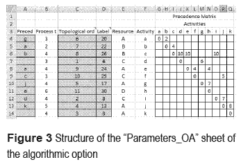
The parameters for the net flow alternative are contained in a spreadsheet, named as Parameters_OA (see figure 3). It contains the description of the activities to be programmed, and their relations with other activities. In its third line, this sheet defines the columns’ headlines, starting to presenting their contents in line 4, as follows: column F contains the ID of the activities; column E identifies the resource in which the activity will be processed; column B registers the processing time of the activity; columns A, C and D are used by the algorithms to solve the problem. So, column C shows the topological order assigned to the activity; column D indicates the finish time of the activity; and column A identifies the node that precedes a given activity on the longest path from the initial one. Said information is useful to reconstruct the critical path of each activity. Columns G and those that follow define the precedence matrix. In this matrix, a value higher than zero in line i and column j means that the activity identified in line i is to be followed by the one identified in column j. For example, a value of 4 in cell L6, corresponding to cell c,f of the mentioned matrix of k*k cell elements, indicates that activity f goes after activity c, and that a minimum of 4 time units after having started the execution of c must have elapsed before starting f. In turn, the inputs in the main diagonal of the matrix correspond to the release times that might exist for activities. To continue with the example, a value of 5 in cell P13, corresponding to input j,j of the matrix, indicates that it is not possible to program this activity until 5 time units have elapsed, regardless of the existence of any precedence constraints that may allow it.

Below is the visual basic code for applications that intend to find the completion time of the activities according to the second approach presented in section 2.3.

1    Sub Algorithmic_option()
2         Call topological_ordering
3         Call label_correction
4    End Sub
5
6    Sub topological_ordering()
7         Dim line, column, activities, Size_L, i, next As Integer
8         Dim did_not_find As Boolean
9         Dim chosen_node, successor_node
10
11      Worksheets(''Parameters_OA'').Select
12
13      'Initiation of variable indegree
14      line = 4
15      While Cells(line, 6) <> Empty
16            Cells(line, 4) = 0
18            line = line + 1
18      Wend
19       actividades = line – 4
20
21       'Calculation of the variable indegree of each activity
22       line = 4
23       While Cells(line, 6) <> Empty 'while there is an activity
24            columna = 7
25            While Cells(3, column) <> Empty
26                If (Cells(3, column) <> Cells(line, 6) And _
27                     Cells(line, column) > 0) Then
28                     Cells(column – 3, 4) = Cells(column – 3, 4) + 1
29                End If
30                column = column + 1
31            Wend
32            line = line + 1
33       Wend
34
35       'Initiation of list L
36       line = 4: Size_L = 0
37       While Cells(line, 6) <> Empty
38            If (Cells(line, 4) = 0) Then
39                'Add to list L,put a list mark in column B
40                Cells(line, 3) = ''*''
41                Size_L = Size_L + 1
42            End If
43            line = line + 1
44       Wend
45
46       'Topological order assignment
47       next = 0
48       While Size_L > 0
49             'Choose a node that belongs to L
50            chosen_node = ''–'': line = 4
51            While chosen_node = ''–''
52                If Cells(line, 3) = ''*'' Then
53                     chosen_node = Cells(line, 6)
54                     Size_L = Size_L – 1
55                     next = next + 1
56                     Cells(line, 3) = next
57                     Cells(line, 4) = "–"
58
59                     'Reduce the value of indegree to the successors of the chosen node
60                     column = 7
61                     While Cells(3, column) <> Empty
62                         If (Cells(3, column) <> chosen_node And Cells(line, column) > 0) Then
63                               successor_node = Cells(3, column)
64                               'Search line of the chosen node's successor
65                               i = 4: did not_find = True
66                              While (did_not_find = True)
67                               If (Cells(i, 6) = successor_node) Then
68                                  Cells(i, 4) = Cells(i, 4) – 1
69                               'If the node has no predecessors, it is added to the list of nodes to be processed
70                               If Cells(i, 4) = 0 Then
71                                  Cells(i, 3) = "*"
72                                  Size_L = Size_L + 1
73                              End If
74                               did_not_find = False
75                         End If
76                         i = i + 1
77                     Wend
78                End If
79                column = column + 1
80            Wend
81            End If
82            line = line + 1
83       Wend
84 Wend
85 End Sub
86
87 'Determines the times elapsed from the initial node to each of the activities
88 Sub Label_correction()
89       Dim line, column, activities, Size_L, i, next As Integer
90       Dim did_not_find As Boolean
91       Dim chosen_node, node_successor
92
93       Worksheets(''Parameters_OA'').Select
94       'Initiation of labels
95       line = 4
96       While Cells(line, 6) <> Empty
97            Cells(line, 4) = 0
98            line = line + 1
99       Wend
100
101     'Scan according to assigned topological order
102     line = 4: did_not_find = True: next = 1
103     While did_not_find
104          If (Cells(line, 3) = next) Then 'found the node with topological order "next"
105              If (Cells(line, 4) = 0) Then
106                   Cells(line, 4) = Cells(line, line + 3) + Cells(line, 2) 'line+3 is the column where r is located
107              End If
108
109              'scan all activities in search of arcs leading to successors
110              column = 7
111              While (Cells(3, column) <> Empty)
112                   If (Cells(line, column) > 0 And Cells(line, 6) <> Cells(3, column)) Then
113                   'Check that d_j < d_i + p_j
114                   If (Cells(column – 3, 4) < Cells(line, 4) + Cells(column – 3, 2)) Then
115                       Cells(column – 3, 4) = WorksheetFunction.Max _
116                                                             (Cells(column – 3, column), Cells(line, 4)) + Cells(column – 3, 2)
117                       Cells(column – 3, 1) = Cells(line, 6)
118                   End If
119              End If
120              column = column + 1
121          Wend
122
123          line = 4
124          next = next + 1
125      Else
126          line = line + 1
127       End If
128
129     If (Cells(line, 6) = Empty) Then
130          did_not_find = False
131     End If
132     Wend
133
134    End Sub

In the lines that follow we present a brief explanation of this implementation. Lines 1 to 4 address the sequential order in which the nodes are processed. The nodes are initially assigned a topological order, and then the label correction algorithm calculates the critical path from the starting node to each of the activities. Lines 13 to 18 show one initiation cycle of variable indegree per activity. Lines 19 to 33 calculate the value of indegree variable for each activity or number of activities that precede it in the graph. Lines 35 to 44 start the list of activities that have no predecessor (indegree value equals zero). Lines 46 to 85 assign the corresponding topological order to the activities in list L. Lines 88 to 134 correspond to the implementation of the label correction algorithm. Lines 95 to 99 assign a value of zero to the label of each activity. Lines 111 to 121 update those activities whose values are lower than the path that leads to them from the node whose variable indegree equals zero. The label correction process includes preceding node information updating, so that it is possible to trace the longest possible path from the initial node to each of the activities of the net.

 

Obtained results

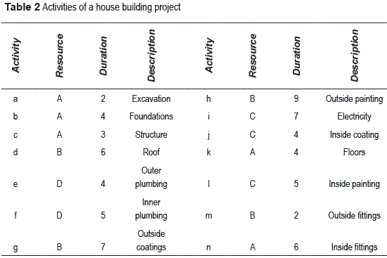
This section presents examples of Gantt charts obtained with the tool here developed. The first represented situation is the activity scheduling of a house building project whose activities with their corresponding description are shown in table 2, as adapted from the version presented by [18] in their chapter about net optimization models.

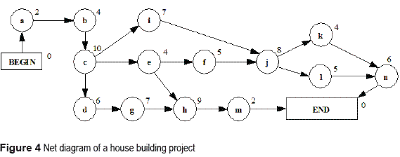
The net diagram corresponding to the house building project presented in table 2, is shown in figure 4.

Once the computer application has been executed, the Gantt chart is obtained as presented in figure 5.

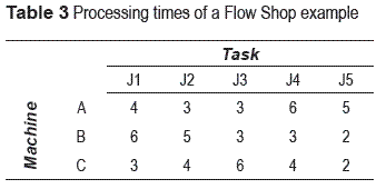
A second application is conducted in production scheduling. The associated Gantt chart indicates the starting times of the different tasks performed in each of the machines of the production workshop. In this sense, table 3 presents the information about a production schedule for a flow shop environment with three machines and 5 tasks, detailing the processing times of the task sequence: j3, j1, j2, j5, j4.

The resulting Gantt chart is presented in figure 6

 

Conclusions and recommendations

The results obtained with the present work can be summarized in the achieving of the objectives proposed, as follows:

1. It offers micro, small and medium sized companies a reliable, rigorous and easily applicable decision making support tool, which is useful for promoting technical solutions in areas such as production and personnel scheduling and project planning, among others.

2. It facilitates non–expert users the application of hard decision techniques – as is the case of optimization – and of easy–to–learn and acquire technologies like SOLVER of Microsoft Excel and VBA macros.

3. It offers students and practitioners involved in the scheduling field, the opportunity to focus on the logic for their solutions methods proposed instead of waste time thinking about how to draw the results obtained.

 

Referencias

1. J. Wilson. ''Gantt Charts: A Centenary Appreciation''. European Journal of Operational Research. Vol. 149. 2003. pp. 430–437.         [ Links ]

2. W. Clark. The Gantt Chart. Ed. The Ronald Press Co. New York (USA). 1925. pp. 84.         [ Links ]

3. J. Herrmann. Handbook of Production Scheduling. International Series In Operation Research & Management. Science. Ed. Springer US. Maryland. 2006. pp. 5–7, 15–16.         [ Links ]

4. H. Gantt. ''A graphical daily balance in manufacture''. ASME Transactions. Vol. 24. 1903. pp. 1322–1336.         [ Links ]

5. F. Taylor. ''Shop Management''. ASME Transactions. Vol. 24. 1903. pp. 1337–1480.         [ Links ]

6. W. Truscott, D. Cho. ''Scheduling batch production with character graphics''. Industrial Engineering. Vol. 19. No. 2. 1987. pp. 17–22.         [ Links ]

7. M. Wennink, M. Salvelsbergh. ''Towards a planning board generator''. Decision Support Systems. Vol. 17. No. 3. 1996. pp. 199–226.         [ Links ]

8. PM Network. ''Project Management Software Survey''. PM Network. Vol. 9. 1995. pp. 35–48.         [ Links ]

9. J. Seyed. ''Right on Schedule''. OR/MS Today. December. 1995. pp. 42–44.         [ Links ]

10. B. Yen, M. Pinedo. On design and development of scheduling systems. Proceedings of the Fourth International Conference on Computer Integrated Manufacturing and Automation Technology. October. 1994. pp. 197–204.         [ Links ]

11. C. Ortiz. ''Implementation issues: a recipe for scheduling success''. IIE Solutions. March. 1996. pp. 29–32.         [ Links ]

12. R. Ahuja, T. Magnanti, J. Orlin. Network Flows. Ed. Prentice Hall. New Jersey. 1993. pp. 193–154, 802–816.         [ Links ]

13. M. Pinedo, X. Chao. Operations scheduling with applications in manufacturing and services. Ed. Mc Graw–Hill. New York. 1999. pp. 2.         [ Links ]

14. ANSI. A Guide to the Project Management Body of Knowledge (PMBOK® Guide) – 2000. Ed. Project Management Institute. Pennsylvania. 2000. pp. 4–7.         [ Links ]

15. E. Balas. ''Disjunctive Programming, Discrete Optimization II''. P.L. Hammer, E.L. Johnson, B.H. Korte. (editors). Annals of Discrete Mathematics. Ed. Elsevier. New York (USA). Vol. 5. 1979. pp. 3–51.         [ Links ]

16. M. Pinedo. Scheduling: Theory, Algorithms, and Systems. Ed. Prentice–Hall. Englewood Cliffs, NJ. 1995. pp. 196, 197, 269–276.         [ Links ]

17. J. Blazewicz, D. Kobler. ''Review of properties of different precedence graphs for scheduling problems''. European Journal of Operational Research. Vol. 142. 2002. pp. 435–443.         [ Links ]

18. F. Hillier, G. Lieberman. Introducción a la investigación de operaciones. Ed. McGraw–Hill Book Company, Inc. México. 1997. pp. 389–395.        [ Links ]