ARTÍCULO ORIGINAL

 

Performance of multivariable traffic model that allows estimating Throughput mean values

 

Desempeño de un modelo de tráfico multivariable que permita estimar el valor medio del Throughput

 

 

Cesar Hernández^1*, C. Salgado², O. Salcedo²

¹Facultad de Ingeniería, Universidad Autónoma de San Luis Potosí. Av. Dr. Manuel Nava no. 8. Zona Universitaria. C.P. 78290 San Luis Potosí, SLP, México.

²Technological Faculty. Francisco José de Caldas District University. Transversal 70 B No. 73 A - 35 Sur. Bogotá, Colombia.

³Engineering Faculty. Francisco José de Caldas District University. Carrera 7 No. 40 - 53. Bogotá, Colombia.

^*Autor de correspondencia: teléfono: + 57 + 311+ 218 6635, correo electrónico: cahernandezs@udistrital.edu.co (C. Hernández)

 

(Recibido el 24 de Septiembre de 2012. Aceptado el 11 de Marzo del 2013)

 

 

---

Abstract

The present paper is aimed at developing a multi-variable traffic model of a Wi-Fi data network that allows estimating throughput mean values. In order to construct the model, data corresponding to an 8-host wireless ad- hoc network were collected using a software package called WireShark; the network was specially designed for modeling purposes. Subsequently, the most convenient multi-variable models were estimated according to the traffic features extracted from the collected data. Results were the evaluated using a software package called STATA, leading to the establishment of significant explanatory variables for the model and its performance levels. For our Wi-Fi network, results show that the analyzed traffic exhibits self- similarity features. Additionally, model coefficients and their corresponding significance levels are shown in various Tables. Finally, an explanatory multivariable model consisting of four variables was produced on the basis of ordinary least-squares methodologies (with a per-cent error of 22.16). The findings suggest that the multi-variable traffic model produced in this study allows a reliable analysis of throughput mean values; however, the model is limited when predicting traffic values for data outside the selected estimation set.

Keywords: Traffic model; multi-variable model; Wi-Fi networks; throughput

---

Resumen

El presente trabajo de investigación tiene por objetivo desarrollar un modelo multivariable de tráfico para una red de datos Wi-Fi que permita estimar el valor medio de throughput; para lograr lo anterior se procedió a capturar los datos correspondientes con el software WireShark de una red inalámbrica Ad Hoc compuesta por ocho host, diseñada e implementada para tal fin. A continuación se estimaron los modelos multivariados más convenientes de acuerdo a las características del tráfico capturado y posteriormente se evaluaron los resultados obtenidos a partir del software STATA, determinando las variables explicativas más significativas dentro del modelo y su nivel desempeño.

Los resultados arrojados por este proyecto de investigación demuestran la autosimilaridad presente en el tráfico capturado de la red Wi-Fi, además, se muestran en diferentes tablas los coeficientes de los modelos y sus respectivos niveles de significancia. Finalmente se desarrolló un modelo multivariado de cuatro variables explicativas a partir de la metodología de mínimos cuadrados ordinarios con un error porcentual del 22,16.

Como conclusión, el modelo multivariado de tráfico desarrollado permite realizar un análisis de los valores medios del throughput con suficientes niveles de confiabilidad, sin embargo, no realiza una buena predicción de los valores de tráfico para datos que estén fuera del conjunto seleccionado para su estimación.

Palabras clave: Modelo de tráfico, Modelo Multivariable, Redes Wi-Fi, Throughput

---

 

 

Introduction

Nowadays communications networks must offer a variety of services in addition to traditional services such as voice and data. The new services include specialized video and audio services together with images, text, control and so on; each of these services requires particular QoS requirements. QoS has become ever more important in terms of service competitiveness in our current society and it represents a compelling aspect regarding the different network requirements in demand [1].

These new characteristics associated to network capacity and network requirements permitted spotting inconsistencies between the traditional models that were based on non-correlated traffic and the behavior (measurements) of the new traffic, particularly regarding correlation-wise structures that appear at different time scales [2].

Since the new traffic behavior of wireless communication networks is too complex to be designed using non-correlated traffic models, it is necessary to develop statistical models that allow forecasting traffic on current communication networks and, for our purposes, forecasting the traffic over a Wi-Fi network, since these networks are widely used and permit easy access to data downloads.

In the last century, network development has involved various proposals for traffic models; each of these models has proved useful in its own particular context. Only until recently - and due to the need for service integration into a single network structure - traffic modeling became a comprehensive research field, where the main goal is to develop predictive models that allow foreseeing the impact of traffic load (from different applications) on network resources and then assess the supply of QoS [2].

The reasons above highlight the importance of having accurate traffic models, therefore the present study attempts to develop a Wi-Fi- network multi-variable traffic model that permits estimating throughput mean values.

Since time intervals between packet arrivals were considered to be independent for the case of a telephone network, it was possible to consolidate a whole mathematical theory that models the effects of such demands on communication limited resources. This is the case of queuing theory, which is widely used when modeling traditional communications networks. The most remarkable contribution from this type of non-correlated models is represented in Erlang loss formula (1); this formula has permitted both designing and scaling telephone networks for almost a century [2].

However, modern communication networks must offer not only voice-and-data services but also many other services (e.g. images, video, audio, text, control and so on). Each of these new services is associated to different criteria in terms of QoS, and so the network should meet different types of requirements.

These new characteristics, in terms of network capacity and network demand, begin to reveal a lack of consistency between traditional models and the actual behavior observed from measuring network performance, particularly when considering correlated structures that extend throughout different time scales. These facts disproved the results obtained from traditional traffic theory, which is based on non-correlated models. The new type of traffic flowing on networks is too complex to be modeled using the techniques that once were successfully applied to telephone networks [2].

Apart from using single-variable models, conventional analysis does not integrate all the relevant information associated with data networks, hence multi-variable traffic models represent a good choice to model data-networks traffic. These alternative models provide a more accurate forecast. Therefore, it has been necessary to develop additional traffic models that permit capturing the greatest amount of significant information possible and considering real traffic features, particularly the existing correlations between arrival-time intervals, which were absent from non-correlated models [2].

When foreseeing the future needs of any complex system, having an accurate traffic forecast is really important in order to define future requirements in terms of capacity and also to plan the possible changes. A very precise model should predict situations in future years, and this very ability represents an advantage when planning future requirements [3].

Therefore, multivariable traffic models are advantageous to: coverage planning, resource reservation, network monitoring, anomaly detection, and the creation of more precise simulation models - in terms of traffic forecast for a given time scale [4].

The present proposal will be presented in a sequential fashion by using four methodological approaches. The first approach is of an exploratory type and is intended to document all the necessary information. The second approach is of a descriptive type and permits detailing each of the characteristics found in the variables of interest. The third approach is of an analytical type and allows defining the influence of each of the variables within the model. The fourth approach is of a predictive type and attempts to apply solutions found in other situations to the context of interest.

 

Metodology

The methodology followed in this study can be described in four stages, namely: traffic generation and traffic capture, Wi-Fi network design and implementation, traffic model estimation and selection, and traffic model evaluation.

Traffic generation and traffic capture

The method to capture the traffic generated in the Wi-Fi network was based on the software package called ''WireShark'', which is an open- source Sniffer that allows capturing all incoming and outgoing traffic through a network adapter (card) installed on a computer [5, 6].

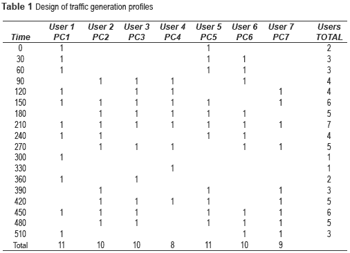
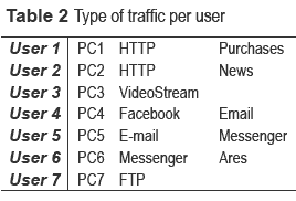
A Wi-Fi network was implemented and a traffic generation pattern was designed for the network. Since the main idea of our study was to build a multivariable traffic model that allowed a more accurate description of current traffic, we decided to analyze the traffic patterns of one entity throughout a complete working day, starting at 8:00 a.m. up until 5:00 p.m. (nine working hours). During this time interval, the behavior of the traffic generated by eight employees was analyzed by observing (on a 30-minute basis) what applications were used on their desktop computers. By using this information, the following step was to emulate the same type of traffic generation through the design of seven independent traffic generation profiles, working for the same nine-hour period (see table 1 and table 2).

The profiles described in table 1 also correspond to the explanatory variables that were initially intended to be included in the model, namely time, number of users and applications. These variables were chosen because (according to the theory) they are closely related with the volume of traffic that is generated within a data network.

Design and implementation of the Wi-Fi network

In order to continue with this study and so meet the remaining objectives, it was necessary to design and implement a Wi-Fi network. Initially, and after studying the characteristics of Wi-Fi networks, it was clear that two possible types of networks were possible, namely infrastructure- based networks and ad-hoc networks [5, 6].

Using an infrastructure-based Wi-Fi network would imply having to capture traffic on each data node (each PC) independently and then put these data together, which requires a big effort in terms of data organization. Hence we decided to implement a Wi-Fi ad-hoc network and set one of the laptop computers as internet gateway; thus all the incoming/outgoing traffic would necessary go through such server. Based on this network and configuration choice, the remaining task was to gather (capture) traffic data in only one computer, namely the server [7, 8].

Once the Wi-Fi network was implemented, local- interconnection and internet-access tests were conducted. Then, traffic capture tests were carried out using Sniffer WireShark. Subsequently, applications were installed on the network nodes (computers) as required (table 2), application tests were also conducted to guarantee proper operation.

Selection and estimation of the traffic model

Once data were captured, it was necessary to export data and organize information using spreadsheets (Excel file). WireShark captures traffic data in real time; on average, WireShark captures a packet every ten milliseconds (10 ms), therefore the number of packets that can be stored in nine hours is extremely large, in this particular case the number of packets was 3,103,201.

For every packet stored, WireShark also saves variables such as the elapsed time (in seconds) after the first capture, the corresponding capture number, the protocol involved, the source and destination IP addresses, the packet size, and a brief description of the information contained in packets [9]. However, the study would not be as meaning full if it were to be based on the direct information provided by WireShark only. The fact that each packet is generated at a single source (IP address) implies that the variable associated to the number of users is always ''1'', and so this value would not be as significant in a multivariable model [10 -12].

Hence, a decision was made to reorganize the data from captured packets by fixing time intervals where all the information within becomes a single traffic datum. The value for the time interval in question was fixed to be one minute so as to obtain consistent pieces of information as well as a representative amount of traffic data. According to the time intervals selected, the initial number of packets (3,103,200) became (9h*60min/h) 540 traffic samples.

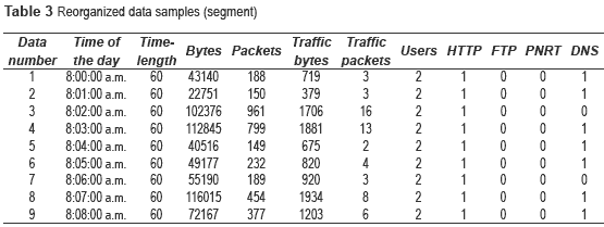
In order to carry out the necessary statistical analysis, the 540 traffic samples were organized as described in table 3.

The first column corresponds to the number of the traffic sample - from 1 to 540. The second column corresponds to the time of the day when the data was captured; this value was obtained from the original Time value, which indicates the amount of elapsed seconds starting at the first capture until the current capture; thus we obtained our values only by adding up the initial time value (eight in the morning). The third column corresponds to the original Time variable. Column 4 holds the number of transmitted bytes during the corresponding one- minute period. Column 5 contains the number of transmitted packets during the corresponding one-minute period. It is worth mentioning that packets are not of the same length, since they come from different applications. If all packets had the same length then perfect co-linearity would exist, and so one of the variables should be eliminated. Column number 6 contains traffic data (dependent variable or explained variable) measured in bytes per minute.

Column 7 corresponds to traffic measured in packets per minute. Usually, measurement units such as bps, Kbps or Mbps, are consider suitable to represent traffic - instead of packets per minute - since the length of packets may vary, and so packets would not represent the exact volume of information flowing throughout the network. Column 8 contains the number of users sending traffic within a given one-minute period. The last four columns show the application protocols being used, namely HTTP, FTP, PNRT and DNS. In these 4 columns, ''1'' indicates that such a protocol was used during the one-minute period; conversely, ''0'' means the protocol was not used. Application layer protocols are considered, since they are directly associated with applications themselves [1].

The protocols that produce the largest amount of traffic regardless of the data are the following: HTTP, FTP, PNRT, DNS, SSL and ICMP; however, SSL e ICMP are not application-layer protocols, thus we focused on the first four protocols mentioned above. The traffic associated to these four protocols accounts for 88% of the whole traffic and their individual percentages are significant, hence it was decided to regard this type of traffic as independent dichotomous variables (defined in a concept framework).

Traffic model assessment

Once the model was estimated, it had to be assessed; initially using 80% of the data that served model estimation, and then using the remaining 20%. This evaluation consisted in determining statistical indices such as adjustment quality [1, 13].

Finally, an estimate of throughput mean values was given based on the proposed traffic model.

 

Analysis and results

The result analysis was divided into six stages, namely: traffic analysis, traffic characterization, traffic-model variables, multi-variable traffic model, traffic-model assessment, and Throughput mean-value estimation.

Traffic analysis

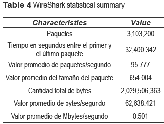
Once traffic had been captured, WireShark yielded a summary of the data (table 4).

According to the distribution of the entire flow of traffic generated by the different protocols, it can be observed that, because of encapsulation processes, each packet (and byte) is counted more than once, depending on the number of protocols involved in each layer of the TCP/IP model.

A packet generated from an FTP application adds not only to the FTP flow (application layer), but also to the TCP flow (transport layer), IP flow (network layer) and Ethernet flow (physical layer).

Hence, the most relevant protocols are: HTTP, FTP, PNRT and DNS. The traffic flow from these protocols accounts for 88% of the application- layer traffic [14].

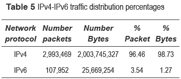
It is interesting to see that some applications are already generating traffic flows using IPv6. Traffic distributions used by both IPv4 and IPv6 can be observed in table 5.

Traffic characterization

The traffic suggests the presence of self-similarity in the traffic that was captured for this study, indicating that the traffic in question is correlated.

Traffic model variables

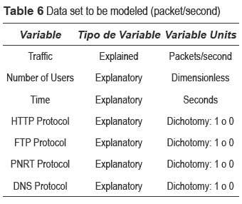
The proposed model is a multi-variable model where traffic represents the dependent (explained) variable, whereas variables such as the number of users, time and application protocols constitute the independent (explanatory) variables (table 6).

According to the captured data, the dependent variable (traffic) can be measured in either packets per second or bytes per second. In the result-analysis stage, traffic measured in packets per second will be considered.

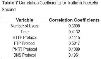
Table 7, shows the results obtained from the correlation analysis between each of the explanatory variables and the explained variable.

The results in table 7 show percentages (decimal fractions) of how much independent variables actually explain the dependent variable; for example, it can be said that the number of users variable explains the variable traffic (measured in packets per second) up to 32%.

The correlation coefficients displayed in table 7 are relatively low for an acceptable model; however, these figures are large enough not to be negligible. Thus it will be worth analyzing the behavior of these variables as a whole.

Multi-variable traffic model

As explained earlier (methodology section), there is only one multi-variable model chosen as suitable for the captured traffic data, namely the panel data model. This model is the one that best fits our context since it permits modeling longitudinal and cross-sectional information data. Cross-sectional means that there is a set of data captured during at the same time, e.g. number of users and protocols. Longitudinal means that there are various data samples along a timeline. If such a timeline were long enough, it would be possible to apply time multivariable models such as VAR and VARMA. However, since variable time in this particular experiment changes on a single-minute basis for nine hours only, the most suitable choice is the panel data model; except for the case of neural networks, which will be reported in future papers [11, 12].

The model to be estimated is described by (2).

Where Trafpaq represents traffic in packets per second, Time, Users, HTTP, FTP, PNRT and DNS are the explanatory variables of the model; i is the variable (sub-index) that indicates the sample set/ captured data, so i takes value from 1 to 540; ε_i represents the non-observable component of the model.

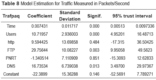
Table 8 shows the results from the model estimation described in ''equation (2)'' - using Ordinary Least Squares (OLS).

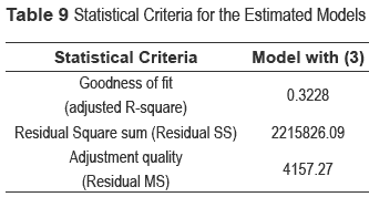
Based on the results in table 8, it is possible to calculate coefficients for each of the explanatory variables, together with their significance level and trust interval. By analyzing the different significance levels, it can be stated that variables HTTP and PNRT are not as significant for this model. According to the results shown in table 8, the estimated model is described by (3) and the table 9 shows the statistical criteria for this model.

Considering now the significance of each explanatory variable within the selected model, the following step was to eliminate non-significant variables and to estimate the model once again. In table 8, it can be observed that variable HTTP, as well as variables PNRT and constant, exhibit low levels of significance within the model; therefore these variables were discarded as negligible. Table 10 shows the results obtained from estimating the selected model without variables HTTP, PNRT, and constant.

Based on the results shown in table 10, it is possible to determine the coefficient of all explanatory variables, as well as their significance levels and trust interval. By analysing significance levels, it can be stated that all the included variables are significant in the model. According to the results shown in table 10, the estimated model corresponds to the description provided by (4), the final model.

Traffic model assessment

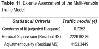
Model assessment was conducted in two stages. The first stage deals with an ex-ante assessment, where only 80% of the captured data were considered; these are the same data that served model estimation. Table 11 shows the results obtained when applying the same statistical criteria (considered in table 9) on these data.

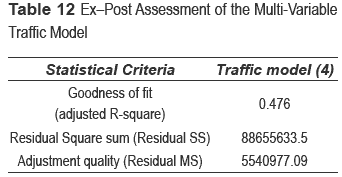
The second stage corresponds to an ex-post assessment, where only the remaining 20% of captured data were considered. These data were not involved in model estimation so as to clearly determine the model's capacity to predict future traffic values. Likewise, table 12 shows the results obtained when applying the same statistical criteria on these data.

As shown in tables 11 and 12, fair comparison parameters are goodness of fit and adjustment quality since these parameters are weighted by the number of samples available, whereas the remaining parameter exhibits significant variations depending on the number of samples (amount of data).

Throughput mean value estimation

According to the multi-variable traffic model already built and described in (4), Throughput mean values can be estimated; to do so, it is only necessary to define a time period in which a particular mean value is to be calculated, then add all traffic values obtained during the same period (in packets per second), and divide this sum by the number of data obtained using the model. The equation (5) summarizes the whole process [15].

In equation (5), i represent a value index of each explanatory (independent) variable.

Comparison with ARIMA model

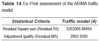
For an even more objective result, it was decided to compare the multivariate model developed with a time series model as ARIMA. To develop the ARIMA model was used Box Jenkins methodology. After performing the corresponding correlograms, the results suggested using an AR (2) and MA (10), from here and after four iterations was obtained performing an ARIMA (1,1,10) described by equation (6).

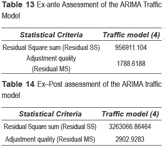
Tables 13 and 14 show the results of the ex-ante and ex-post, following the same methodology used above, these results can be compared with those in tables 11 and 12.

A comparison of the results in tables 13 and 14, shows a better performance of the models based on time series regarding multivariate linear models, this performance is about 43% better.

 

Conclusions

The multi-variable traffic model presented permits analyzing throughput mean values at reliable levels; however, the model is unable to produce accurate predictions of future traffic values for data outside the selected estimation data set.

Although it was clear from the results that a large percentage of the generated traffic was associated to HTTP and PNRT, the impact of these two protocols was not as significant within the model itself. This might be explained by considering that protocol HTTP is very often present in the generation of current Internet traffic and also that most applications use P2P in the case of PNRT.

After plotting the traffic generated by the Wi- Fi network using different time scales, - both in packets per second and in bytes per second - it was clear that self-similarity patterns were present in each representation. This reinforces the ideas found in current studies about modern traffic characterization.

Although both the traffic measured in packets per second and the traffic measured in bytes per second are relatively important when planning and controlling data networks, the first sort of units (packet per second) adjust better to explanatory variables than the latter.

There are some of the disadvantages to the multi­variable traffic models such as the one presented in this study, particularly when estimating the model itself; namely determining independent variables, which are not easy to model. This suggests that there is a comprehensive field of research topics that need to be studied regarding traffic models. The results of the present study demonstrate how important it is to use correlated models when modeling Internet traffic on a wireless data network.

 

References

1. C. Hernández, O. Salcedo, A. Escobar. ''An ARIMA model for forecasting Wi-Fi data networks traffic values''. Revista Ingeniería e Investigacion. Vol. 29. 2009. pp. 65-69.         [ Links ]

2. M. Alzate. ''Modelos de tráfico en análisis y control de redes de Comunicaciones''. Colombia Ingeniería. Vol. 9. 2004. pp. 63-87.         [ Links ]

3. M. Tiep, G. Bidisha, W. Simon. ''Multivariate short- term traffic flow forecasting using Bayesian vector autoregressive moving average model''. Transportation Research Board. Vol. 12. 2012. pp. 16.         [ Links ]

4. M. Papadopouli, H. Shen, E. Raftopuulos, M. Ploumidis, F. Hernández. Short-term traffic forecasting in a campus-wide gíreles network. in IEEE 16^th International Symposium on Personal, Indoor and Mobile Radio Communications. Berlin, Germany. 2005. pp. 1446-1452        [ Links ]

5. D. Mark, R. McDonald, R. Antoon. Aspectos Basicos de Networking. Ed. Cisco Press. Madrid, España. 2008. pp. 606.         [ Links ]

6. P. Fierens. Introducción a las Redes Wi-Fi. Instituto Tecnológico de Buenos Aires. Boletín electrónico: Comisión Intramericana de Telecomunicaciones. No. 14. Agosto. 2005.         [ Links ]

7. N. Torres, L. Pedraza, C. Hernández. ''Redes neuronales y predicción de tráfico''. Tecnura. Vol. 15. 2011. pp. 90-97.         [ Links ]

8. J. Sa Silva, R. Ruivo, T. Camilo. IP in wireless sensor networks Issues and lessons learnt. In Proceedings of the 3^rd International Conference on Communication Systems Software and Middleware and Workshops. Bangalore, India. 2008. pp. 496-502.         [ Links ]

9. A. Feria. Modelo OSI. Ed. El Cid Editor. Santa Fe, Argentina. 2009. pp. 14.         [ Links ]

10. G. Box, G. Jenkins, G. Reinsel. ''Forecasting and Control''. Time Series Analysis. 3^rd ed. Ed. Prentice- Hall. Englewood Cliffs. San Francisco, USA. pp. 75. 1994.         [ Links ]

11. Y. Chia, J. Shyu. ''Applying multivariate time series models to technological product sales forecasting''. International Journal of Technology Management. Vol. 27. 2004. pp. 306-319.         [ Links ]

12. M. Ariño, P. Franses. ''Forecasting the levels of vector autoregressive log-transformed time series''. International Journal of Forecasting. Vol. 16. 1999. pp. 111-116.         [ Links ]

13. J. Carroll, C. Hernández. ''Comparación del modelo FARIMA y SFARIMA para obtener la mejor estimación del tráfico en una red Wi-Fi''. Tecnura. Vol. 16. 2012. pp. 84-90.         [ Links ]

14. A. Dainotti, A. Pescapé, P. Rossi, F. Palmieri, G. Ventre. ''Internet traffic modeling by means of Hidden Markov Models''. Computer Networks. Vol. 52. 2008. pp. 2645-2662.         [ Links ]

15. K. Balaji. Forecasting models and adaptive quantized bandwidth provisioning for nonstationary network traffic. PhD. Dissertation. University of Missouri. Kansas City, United States. 2006. pp. 173.         [ Links ]