


Services on Demand
Journal
Article
 English (pdf)
 Article in xml format
 Article references
 Send this article by e-mail
Indicators
-
 Cited by SciELO
 -
 Access statistics
Related links
-
 Cited by Google
 -
 Similars in
SciELO
Similars in
SciELO -
 Similars in Google
Share

 Permalink
Revista Facultad de Ingeniería Universidad de Antioquia
Print version ISSN 0120-6230
Rev.fac.ing.univ. Antioquia no.68 Medellín July/Sept. 2013
ARTÍCULO ORIGINAL
A simplification to the fast FIR-FFT filtering technique in the DSP interpolation process for band-limited signals
Una simplificación a la técnica de filtrado rápido FIR-FFT en filtros de interpolación digital para señales limitadas en banda
Francisco Rubén Castillo Soria1*, Ignacio Algredo Badillo1, Gustavo Fernández Torres2, Jaime Sánchez García3
1Computer Engineering Department, UNISTMO University, Av. Universidad S/N. CP. 70760. Tehuantepec, Oaxaca, México.
2Petroleum Engineering Department, UNISTMO University, Av. Universidad S/N. CP. 70760. Tehuantepec, Oaxaca, México.
3Department of Electronics and Telecommunications, CICESE Research Center, Carretera Tijuana-Ensenada 3918. CP. 22860. Ensenada BC, México.
*Autor de correspondencia: telefax: + 52 + 971 + 52 24 050 ext. 116, correo electrónico: frcsoria@bianni.unitsmo.edu.mx (F. Castillo)
(Recibido el 16 de Febrero de 2012. Aceptado el 5 de Agosto de 2013)
Abstract
Frequently, when great amounts ofsampled data are manipulated, it is necessary to reduce them to a fraction that truly represents the data. Here two elements are important; neither is it desirable for the amount of data to be too extensive; nor is it desirable to lose key information. For the data econstruction,it is often required a interpolation technique. This work proposes an optimization of the fast FIR filtering-based DSP interpolation technique. The resulting interpolator is a feasible, simplified version of hardware implementations, which is ideal for the reconstruction of band-limited signals with adequate sampling. In case studies included in this work, wind and temperature signals are used. The temperature signal has a suitable sampling rate and with the use of the interpolator it presents an error of 3.95% for a reduction of 99.61% of the data. The wind signal is very unpredictable and it does not have a suitable sampling rate. Hence, the interpolator does not improve the reconstruction of the signal in comparison to the averages. Typically, an average signal value is recorded for each 10 minute period, in which, the wind signal presents an error 8.6 times greater than the temperature signal. In order to reduce this error in the wind signal, it is recommended to increase the sampling rate and the quantization levels in measurement equipment.
Keywords: DSP Interpolation, sampling, fast FIR filtering, decimation
Resumen
En ocasiones cuando se manipula una gran cantidad de datos muestreados, se requiere reducir dicha cantidad para conservar solo una representación de estos. Aquí dos aspectos son importantes; por un lado no se quiere que la cantidad de datos sea demasiado extensa y por el otro no se quiere perder información. Para la reconstrucción de datos generalmente se requiere de una interpolación. En este trabajo se presenta una optimización a la técnica de interpolación digital basada en el filtrado rápido FFT. El interpolador resultante es una versión simplificada factible de implantaciones hardware, que resulta ideal para la reconstrucción de señales pasa-bajas, con muestreo adecuado. Como casos de estudio se utilizan señales de viento y temperatura. La señal de temperatura, tiene un muestreo adecuado y con el uso del interpolador presenta un error de 3.95% para una reducción del 99.61% de datos. La señal de viento es caótica y no tiene un muestreo adecuado por lo que el interpolador no mejora la reconstrucción de la señal en comparación a los promedios. Típicamente estas señales se almacenan en promedios de 10 minutos, en las cuales, la señal de viento presenta un error 8.6 veces mayor que la señal de temperatura. Para reducir este error en la señal de viento es recomendable aumentar la velocidad de muestreo y los niveles de cuantización en equipos de medición de dicha señal.
Palabras clave: Interpolación DSP, muestreo, filtrado rápido, FFT, decimación
Introduction
In the modern world, digital systems are indispensable tools, but efficiency in time and space requirements is a must. Algorithms or processes generating high throughputs and using few storage resources should be implemented. There are many ways to improve these requirements, such as optimal algorithms, faster computers and bigger storage devices. In the latter, sampling is important because it determines an adequately small group from the total number of target population, which warrants generalization without storing much data.
When signals are going to be sampled, it is important to determine the amount of data that must be stored in a way that the required database does not become too extensive, while also preserving information contents. In any case, if information is lost, it is desirable to know the amount of that error.
For limited-band signals, the Nyquist theorem establishes a lower limit on the sampling frequency [1]. This limit sets a necessary condition for the correct reconstruction of the signal. If the sampling rate is below this limit, information content is lost in a definitive way. This phenomenon is known as aliasing. On the other hand, if there is an oversampling, then there is a great amount of data which is redundant, because it does not add useful information.
When designing sampling and reconstruction systems, even though the sampling may be correct, the implementation of reconstruction methods is not always an easy task. This problem is directly related to the implementation of the reconstruction filters (interpolation) [2, 3]. On the other hand, in addition to these details, the real signals occasionally present a spectral content that makes it difficult the right implementation of the sampling theorem. It has been demonstrated that for these kind of signals, the ideal filter based on sinc(x) type functions is no longer optimal [4, 5].
In digital systems, the common technique to get values between two samples where there is no information is known as DSP (Digital Signal Processing) interpolation. DSP interpolation is based on the use of digital filters for the reconstruction of the signal with a previous stage of sample insertion. Typically, the interpolation filters are designed specifically for each signal so that smaller errors are obtained. Among the interpolation techniques, the zero stuffing in combination with a low pass filter is typically utilized [6, 7].
The signals measured in meteorological stations such as wind and temperature are typically sampled at regular 10 minutes intervals, with the aim for the stored data to fit in the minimum space [8]. Nevertheless, it is important to highlight that according to the sampling theorem, the signals with major spectral contents must be sampled at a greater speed than those that have a reduced spectral content. If this characteristic is not taken into account, information in stored data could not be good enough to reconstruct the original signal. On the other hand, if the signal is oversampled, a good signal reconstruction is obtained but with an unnecessarily large amount of data.
In any case, for a right utilization of the data, one must know: i) the magnitude of the error in stored data, ii) the best interpolation technique for those data and iii) the error caused by each technique used. The methodology presented in this work can be used to determine the sampling characteristics as well as a suitable reconstruction method whenever a correct sampling rate is used. This technique can be applied for the analysis of other band limited signals in real applications.
DFT-based interpolation
Decimation is a process often employed by designers to decrease the sampling rate by extracting samples of a signal. The decimation is based on undersampling applied to the input signal. When an increase in the sampling rate is required, interpolation is used. This process makes an estimation of the values of the added samples, see figure 1.
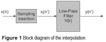
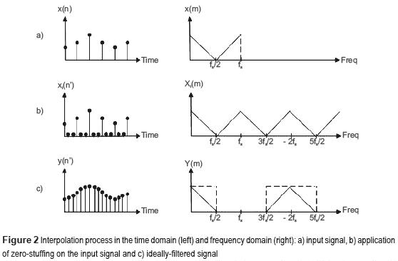
In digital systems this process is known as DSP interpolation. Considering the original signal (see figure 2a) the interpolation process has two stages. The first one consist in carrying out sample insertion, (zero stuffing, see figure 2b) the purpose of which is to increase the sampling speed. In the second stage, the obtained signal is fed into the low-pass filter, removing the frequency components (images) which are not desired.
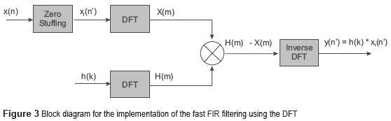
For the low pass filter stage, one of the most commonly used techniques is the FIR (Finite Impulse Response) filter. This technique can be implemented in the so called Fast FIR Filter using FFT. Since the convolution in the time domain corresponds to multiplication in the frequency domain, the filtering operation can be realized by using the scheme shown in figure 3. Initially, the spectra of the signals are obtained. This is done by using the DFT for both the input signal x(n) and the filter response h(k). Afterwards, a multiplication is carried out in the frequency domain (convolution in time domain) and finally, the IDFT (inverse DFT) is applied to return to the time domain, obtaining y(n').
In several studies, it has been demonstrated that these in the time domain whenever the output sequence filters are faster than the filters using convolution y(n') has a size greater than 30 taps [6].
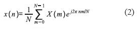
Both transforms, DFT (1) and IDFT (2), are discrete versions of the Fourier transform. The first is used to obtain the spectral characteristic in the frequency domain, and the second is utilized to return to the time domain. For a given signal x(n), the DFT in exponential form is described as:
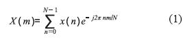
the IDFT in exponential form is described as:
where:
m,n: Frequency and time indexes, respectively
X(m): the mth DFT output component
x(n): the input sequence
N: the number of samples of the input sequence.
Proposed methodology
The interpolator performance is directly related to the filter design. The design of the ideal filter becomes more complicated when its implementation is in the time domain (see figure 2) because the function h(k) = sinc (k), in theory, would have an infinite size. This is another advantage of the filter implementation in the frequency domain. The Fourier transform of the function h(k), is described in (3):
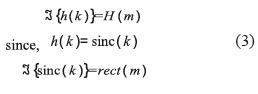
Therefore, for the function rect(m), a uniform content of frequencies in all the rank is present. In this case, H(m) =1, so that the multiplication with H(m) is avoided in the process.
Usually, when the direct and inverse FFT are used both have the same length and they depend on the sequence lengths h(k) and x(n), so that if h(k) is of length P and x(n) is of length Q, the length of the final sequence y(n') will be P+Q -1. So, to use fast convolution an N-point FFT size must be chosen such that N≥(P+ Q - 1) and zero pad h(k) and x(n) so they have a new length equal to N. In this way, zero-stuffing can be avoided, and it is possible to reduce the computational burden.
When these considerations are established, a simplified version of the interpolator is obtained as shown in figure 4, where the use of the FFT is also proposed.
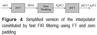
The interpolation process is reduced to the following steps:
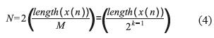
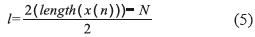
1. Calculate X(m), which is obtained from applying the FFT of the M-order decimated signal x(n), using N equal to twice the length of the input sequence divided by M, (4). Furthermore, it is required that M=2k with positive integer k,
2. Zero pad. Eq. (5) shows the quantity l, of added zeros at each end of the signal X(m).
3. Compute the IFFT, applying it to the signal with zero-padding to obtain the interpolated signal y(n') in the time domain.
4. Trim the signal y(n').
The response of a smooth filter such as the proposed one is optimal for the signal reconstruction when the signals have been correctly sampled (according to the Nyquist theorem). Nevertheless, in real signals this does not always happen.
Generally, before implementing any filter, the designer should know the characteristics of the sampled signal.
Implementation
For the study presented in this work, the wind and temperature signals are used. This data was obtained from the meteorological station of the Unistmo University, corresponding to one week of January 2009.
An implementation was developed in the Matlab programming language, establishing sequences of 8192 samples, using a decimation of 2 ≤ M ≤ 256 for M = 2k with the positive integer k as the FFT requirement. For the extreme case M = 256, only 32 samples of the 8192 original ones are preserved. This happens for both temperature and wind signals.
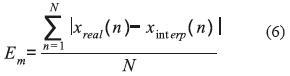
As a measurement of the reconstruction error, a definition of the average error is used, see Eq. (6).
Temperature signal
8192 measured values are considered each minute, as this is the fastest sampling available. Typically, 10-minute averages are used. The environmental temperature signal varies from 17 to 33.3 °C and the resolution is 0.1 °C. This is the reason why each sample can have a quantization error of up to 0.05 °C.
Using the proposed methodology, figure 5 shows the waveforms through the entire process. Figure 5a shows the temperature signal in its original form (time domain).This signal is decimated, using M = 128, see figure 5b, and its FFT transformation is presented in figure 5c. Finally, the signal is reconstructed in the time domain. The signal processed by FFT presents greater amplitudes, which are focused on the center frequencies, and few variations of spectral components are directed towards the highest frequencies.
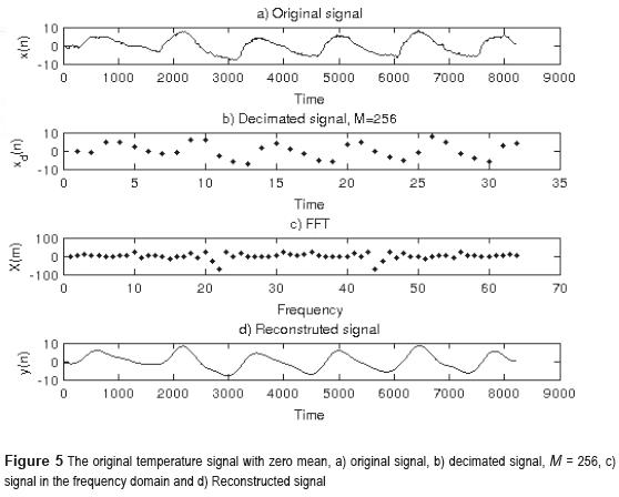
Figure 6 shows the reconstructed signal compared to the original temperature signal with decimation order of M = 16. The samples shown are from 4400 to 4560.
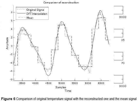
Figure 7 shows the measured error for the temperature signal. For the decimation order M ≤ 8, the averaged signal has a slightly smaller error than the filtered signal. For the decimation with M ≥ 16, the interpolator has a considerably smaller error in comparison to the averaged signal.
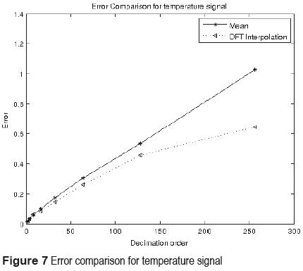
Evaluating these results, for the case of the temperature signal with interpolation M = 256, the expected average error is approximately 1°C, otherwise, if the interpolator is used, the error is 0.6434 °C. If this last error is admissible, it means that the amount of data can be reduced from 8192 to 32 samples. For the dynamic range, this error represents the 3.94%, and a data reduction of 99.61%.
Wind signal
The wind signal varies from 0 to 11 m/s and has a resolution of 0.5 m/s, so each sample can have a quantization error of up to 0.25 m/s.
Applying the proposed methodology, the wind signal is processed and analyzed giving the results shown in figure 8. There, several waveforms are presented: the wind signal in its original form in the time domain (see figure 8a), the decimated version for M = 128 (see figure 8b), the spectral components computed by FFT (see figure 8c), and the reconstructed signal (see figure 8d). In comparison with the temperature signal, the wind signal's spectral components have a smaller amplitude towards the center fequencies. Nevertheless, spectral components in higher frequencies are present, which implies that thewind signal is not correctly sampled.
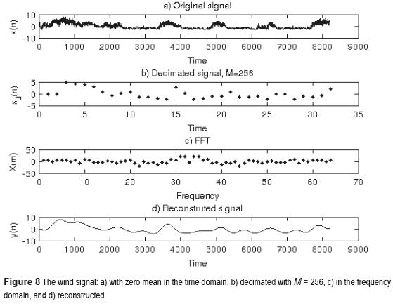
Figure 9 shows the reconstructed signal by using the filter and averages compared to the original wind signal. The decimation order is M = 16 and samples from 4100 to 4600 are shown. For the wind signal, a significant quantization error can be measured.
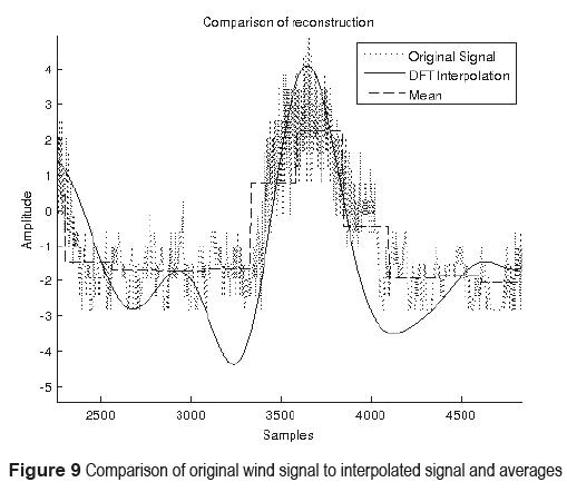
Figure 10 shows the measured error for the wind signal. For the decimation with order M = 2, the interpolator presents a smaller error in comparison with the averages, although, for decimation with orders M ≥ 4, the averages have a smaller error, compared to the interpolator results.
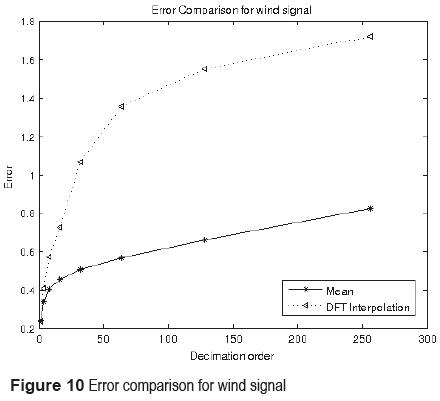
If averages in the reconstruction are used, the amount of data can be reduced from 8192 to 32 samples, reporting an error of 0.8231 m/s. For the dynamic range considered, this error represents 7.69 %. For the same case, the interpolator gives an error twice as big as those shown in the averages. The error cannot be reduced by the interpolator because the wind signal has not been correctly sampled.
Results
The temperature signal behaves smoothly in the time domain, and its FFT version shows that a greater amount of energy is concentrated around the low frequencies. In this case, the reconstruction was improved by using the FFT fast filtering technique of interpolation, and its error was reduced when compared to the results of the averages.
On the other hand, the wind signal shows random behavior and its FFT version reports that there are frequency components over the whole range, which makes it evident that the sampling is not good enough. For this signal, a better reconstruction can be achieved by using the interpolator for a single value (N = 2). On the other hand, for N≥ 4, a reduced error is obtained when averages are used.
Considering averages of 10 minutes, the wind signal presents an error, which is five times greater than the temperature error signal. When the interpolator is used, the temperature signal error is reduced by around 12%, whereas the wind signal error increases to 32%. According to the sampling theorem, the signal must be sufficiently sampled for its correct reconstruction. These results show that although both signals are sampled at the same rate, the temperature signal is sampled better than the wind signal.
Conclusion
The fast filtering FFT interpolator constitutes an effective tool for the reconstruction of low-pass signals, which have been sampled within the limits of, or very close to, the Nyquist theorem, reducing the error in comparison to the averages, which are traditionally used. The filter performance for the temperature signal is satisfactory. The small variations with low-order interpolation can be attributed to the poor quantization of the signal.
According to the analysis, the use of the proposed methodology reveals that the wind signal has been under-sampled in addition to showing poor quantization. In this case, a better approximation is obtained by using averages. However, it is difficult to get a precise result because of the lack of a reference point. By using the interpolator, a better reconstruction is achieved when the decimation with order M = 2 is used, i.e. when the sampling rate is greater. For the wind signal, a considerable error is present due to the deficient quantization, affecting the analysis by making distortions to the original signal. Therefore, it is recommended to use measurement equipment for the wind signal with a greater sampling rate. It is also suggested to use a greater resolution in order to reduce the quantization error in the measurements.
Acknowledgements
We would like to thank the professors Michael Garton and Timothy Lamb for their help in proofreading this paper. We would also like to express our gratitude to the people responsible of the meteorological station at the University of the Istmo for providing us with the measured data.
References
1. J. Proakis, D. Manolakis, Digital Signal Processing. Digital Signal Processing, Principles, Algorithms and Applications. 4th ed. Ed. Pearson, Prentice Hall. New Jersey, USA. pp. 26-30 [ Links ]
2. C. Herley, P. Wong. ''Minimum Rate Sampling and Reconstruction of Signals with Arbitrary Frequency Support''. IEEE Transactions On Information Theory. Vol. 45. 1999. pp. 1555-1564. [ Links ]
3. V . Kazakov, S. Afrikanov. ''Sampling - Reconstruction Procedure of Gaussian Fields''. Computación y Sistemas. Vol. 7. 2006. pp. 227-242 [ Links ]
4. T. Strohmer. 'Implementations of Shannon's Sampling Theorem: A Time-Frequency Approach''. Sampling Theory in Signal and Image Processing. Vol. 4. 2005. pp. 1-17. [ Links ]
5. F. Castillo, J. Arellano, S. Sánchez. ''Statistical Approach to Basis Function Truncation in Digital Interpolation Filters''. International Journal of Electrical and Electronics Engineering. Vol. 4. 2010. pp. 229-233. [ Links ]
6. R. Lyons. Understanding Digital Signal Processing. 1st ed. Ed. Prentice Hall. New Jersey, USA. 2004. pp. 515-516, 387-389 [ Links ]
7. R. Aboul, S. Bozic. ''Multirate Techniques in Narrow Band FIR Filters''. International Journal of Electronic. Vol. 71. 1991. pp. 939-949. [ Links ]
8. H. Mattio, F. Tilca. Recomendaciones para Mediciones de Velocidad y Dirección de Viento con Fines de Generación Eléctrica, y Medición de Potencia Eléctrica Generada por Aerogeneradores. Secretaría de Energía. Buenos Aires, Argentina. 2009. pp. 3-4. [ Links ]
