ARTÍCULO ORIGINAL

Application of Airborne LiDAR to the Determination of the Height of Large Structures. Case Study: Dams

Aplicación del LiDAR aerotransportado a la determinación de la altura de grandes estructuras. Caso de estudio: Presas

Rubén Martínez Marín^*, Juan Gregorio Rejas Ayuga, Miguel Marchamalo Sacristán

Laboratorio de Topografía y Geomática, Dpto. Ingeniería y Morfología del Terreno, Universidad Politécnica de Madrid. CP. 28040. Madrid, España.

^*Autor de correspondencia: teléfono: + 34 + 91 + 3366670, correo electrónico: ruben.martinez@upm.es (R. Martínez)

(Recibido el 16 de junio de 2013. Aceptado el 23 de enero de 2014)

Abstract

The best way to determine the height of dams is to level the top of the dam applying a geometric leveling. Nevertheless this task is very demanding and expensive. The accuracy potential of LiDAR (Light Detection and Ranging) data has significantly improved. These systems can provide accuracy of 2-3 cm level, which could be enough to be applied in the determination of the height of dams. The point acquisition density is an important factor involved in the process of determining the height using LiDAR technique. Finally, since the LiDAR technique is based on ellipsoidal heights, the coordinates must be transformed to the official orthometric system. This paper shows the results obtained using low density airborne LiDAR data (0.5 pts/m²) and their validation with post-processed GPS (Global Positioning System) observations. Test results have shown LiDAR can be accurate enough (10-25 cm) to determine the height and to be applied in many civil engineering activities.

Keywords: Accuracy, airborne LiDAR, low density LiDAR, dam height

Resumen

La mejor forma de calcular la altura de una presa es realizar una nivelación geométrica de precisión. No obstante, este método es demandante y costoso. La precisión de los datos obtenidos ha mejorado sustancialmente, esta tecnología puede proveer precisiones de 2 a 3 centímetros, más que suficiente para determinar la altura de presa y utilizar ésta como dato de partida para cualquier actividad posterior que así lo requiera. La densidad de adquisición de los datos LiDAR (Light Detection and Ranging) es importante para establecer la bondad de los resultados. Finalmente, como los sistemas LiDAR aerotransportados están basados en alturas elipsoidales, es necesario transformarlas a ortométricas. Este trabajo muestra los resultados obtenidos usando un LiDAR de baja densidad (0.5 pts/m²) y su validación con observaciones GPS (Global Positioning System) en postproceso. Los resultados demuestran que se puede obtener una precisión del orden de 10-25 cm, suficiente para la mayoría de las actividades relacionadas con la ingeniería civil.

Palabras clave: Precisión, LiDAR aerotransportado, LiDAR de baja densidad, altura de presa

Introduction

Lately, the deployment and application of LiDAR (Light Detection and Ranging) systems has undergone enormous growth. Efficiency and affordability have made LiDAR a primary tool for collecting a variety of high quality surface data in much shorter periods of time than previously possible for multiple purposes [1-3]. In addition, hardware LiDAR technology has also been improved, in particular the pulse rate frequency increased significantly; while earlier systems provided 33 kHz pulse rate, state-of-the-art LiDAR systems are capable of providing pulse repetition rate of up to 100 kHz. Furthermore, the ranging accuracy improved to 2-3 cm level, and the availability of intensity signal became common [4]. These developments resulted in improved data quality in terms of higher point density and better accuracy, which in turn, opened new application areas of LiDAR [5]. Modern LiDAR systems with the cm-level ranging accuracy and high pulse rate, in theory, could be applied to topography works, such as leveling processes [6], even more, ground- based LIDAR systems are being used to monitor movements of large structures and landslides, as a complement of other instruments, for instance, non-prism total station [7].

However, besides the laser ranging error there are several potential error sources that can degrade the accuracy of the acquired data. LiDAR systems are complex multi-sensor systems, and incorporate at least three main sensors: the GPS (Global Positioning System) and INS (Inertial Navigation System) navigation sensors; and the laser-scanning device (see figure 1).

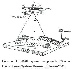
There are multiple causes of errors that affect the process: navigation errors; individual sensor calibration or measurement errors; and inter-sensor calibration errors or a misalignment between the different sensors [8].

Those kinds of errors can be minimized applying a rigorous system calibration, but there are always discrepancies between the reality and the acquired data. Nevertheless, the accuracy achieved with this system is good enough to be applied to most of the common civil engineering activities.

Recently, many methods have been developed to measure the accuracy of the acquired data [9-11]. The main conclusion is that the vertical accuracy is higher than the horizontal. In other words, horizontal errors in LiDAR data are usually more significant [12] than vertical errors.

According to the latest studies, the positioning accuracies obtained, using optimal targets and different LiDAR points densities, may be from 2.0 cm to 15.0 cm [13-15]. Table 1 shows the most representative values obtained.

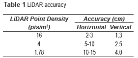
Obviously, the greater the density the better the results, however investing more resources and increasing the total cost. When using a density close to 1.78 pts/m², high accuracies can be expected, 4.0 cm error at vertical positioning, but a lower density, 0.5 pts/m² (the official airborne LiDAR in Spain) without any optimal target in field, was managed.

In spite of the fact that the best way to calculate the dam height is, without a doubt, to level the top of the dam applying a geometric leveling, for some civil activities, where high accuracy is not necessary, but the economy is very important, the use of public data LiDAR can help to achieve good results. The main goal of this study is two-fold, firstly to determine whether or not that low density LiDAR data set is suitable to be used to calculate the dam height and secondly, the accuracy obtained applying the proposed methodology.

The research reported in this paper presents a contribution to calculate the dam height using standard LiDAR data (low density) and the official geoid height model applied to the dams managed by Canal de Isabel II (Madrid-Spain) in the first phase, comparing the results with the data obtained using post-processed GPS data, in the second phase.

Methodology

Raw LiDAR data

The LiDAR dataset used in this research belongs to the PNOA (Plan Nacional de Ortofotografía Aérea) Spanish project that is currently being carried out. The main PNOA project characteristics (see www.ign.es/PNOA ) are as follows:

- Grid step size: 1.41 m x 1.41 m

- Digital Terrain Model accuracy: RMSE (Root Mean Square Error) ≤0.15 m

- Density: 0.5 pts/m² (low density)

- Format file: ''LAS'' binary format (LiDAR standard format)

- Coordinate system: ETRS89 (European Terrestrial Reference System 1989)

- Free of charge for users

Among the dams managed by Canal de Isabel II (Comunidad de Madrid-Spain), thirteen dams were selected to be studied. The first work was to locate, at least, one reference mark and one base near the top of each dam to be able to install the reference and the rover GPS in order to calculate the coordinates of the reference mark.

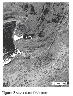
Once the reference marks were built and their coordinates known, twenty two tiles were extracted from the LiDAR dataset. Each tile is a square of 2.000 m x 2.000 m, containing over 2.000.000 points (see figure 2).

Reference marks (control points)

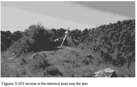
The coordinates of control points located at the crest of the dams, were calculated applying a usual DGPS technique (see table 2). The following process was made for each dam: a GPS receiver (Leica GPS1200. See figure 3) installed at the base point near the dam, was observing for at least two hours. Coordinates of the base were calculated in post-process taking corrections from the permanent stations that the Comunidad de Madrid has installed. The rover GPS (Leica GPS1200) installed at the reference mark (crest of the dam) received corrections from the static GPS located at the base point and the reference mark coordinates were calculated also in post- process. Those coordinates have been considered as ''real coordinates'' in order to be compared with results obtained using LiDAR data.

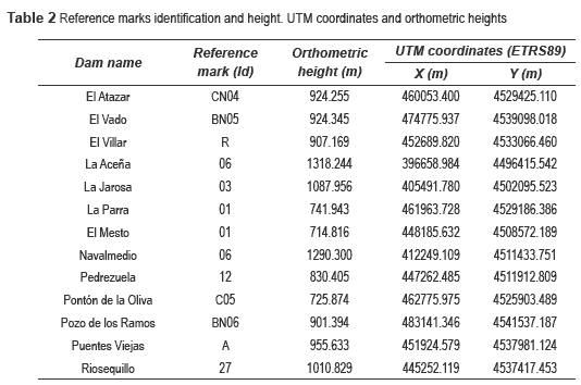
Since the coordinates calculated with GPS are referenced to the WGS84-ETRS89 (World Geodetic System 84 / European Terrestrial Reference System 1989) system, a coordinate transformation was needed in order to obtain the orthometric heights. To solve that problem, the official Spanish Geoid (EGM08-REDNAP), issued by the Instituto Geográfico Nacional (IGN), was applied (see www.ign.es).

Filtering LiDAR data

A customized program was developed in order to select the coordinates of each topographic reference marks located on the crest of the dams (see figure 4). That program has several possibilities:

- Select a rectangle to rule out any point situated outside of it.

- Set up the influence radius in order to search points only in that circle.

- Remove any point with a height larger than a given value.

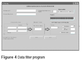
For each dam, knowing the reference mark coordinates and using the filtering program, a subset of LiDAR points were extracted to obtain only points near the reference mark. In this step, proximity criterion was applied.

Calculating reference mark coordinates with LiDAR data

Since there are no points belonging to LiDAR subset (filtered) where planar coordinates match with the real coordinates (observed with GPS), a procedure was applied in order to estimate the X-Y coordinates and then assign the Z coordinate. The procedure consisted in taking the LiDAR points around the reference mark (in 2D, distance equal or less than 1.0 m) and to apply a gravitational interpolation, to estimate the Z coordinate.

Starting from the X-Y coordinates of the reference mark, a subset of LiDAR points is extracted from LiDAR files using the filtering program. From this subset, a new selection criterion is applied using equation (1):

Given a reference mark RM (x_RM, y_RM, z_RM), being (x_RM, y_RM, z_RM) real coordinates obtained from GPS, a point P(x_p, y_p, z_p) is selected when distance from P to RM is equal or less than 1.0 m, that is:

Assuming that there are n points in the LiDAR subset, the estimated Z coordinate height (Z'_RM ), is given by the expression (2):

Where,

Z'_RM is the estimate Z coordinate for the reference mark given

z_i is the Z coordinate of point i

D_i^RM is the Euclidean distance from point i to RM

Results

Table 3 shows the differences between the GPS heights and the corresponding results obtained with LiDAR. Almost all of them are negatives, that is, GPS height is larger than LiDAR height, except four cases highlighted with asterisk and only one with double asterisk (higher discrepancy) that will be discussed later in the next section.

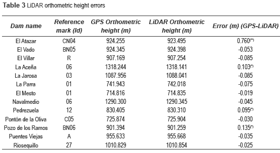
Error was always measured by subtracting the LiDAR from the GPS elevation, resulting in positive errors for an under-prediction of the orthometric height. Several measures of error were computed: mean signed error (table 3), mean absolute error and RMSE. The RMSE was computed by the expression (3):

and the MAE (mean absolute error) by equation (4):

Where,

Z_GPS are the orthometric heights (m) from the GPS

Z_LiDAR are the orthometric heights (m) from LiDAR

n is the number of reference marks observed

Discussion

The main objective in this study is to validate LiDAR dataset as a good source of information to determine the height of a dam suitable to be applied in many civil engineering activities. The results show that the mean absolute error is less than 12.00 cm and the root mean square error is less than 22.30 cm. With these values we can affirm that it is viable to apply this methodology to determine the height. Nevertheless there are some results that are positive, while the majority are negative and small. To find out why that happens, we had to visit the dams again, and look for the reference marks (figures 5 and 6 show some mark locations).

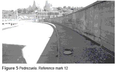
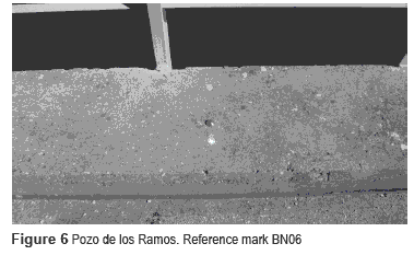
All figures show the same characteristic (see Figures 5 and 6), the reference marks are on the sidewalk or over a concrete base, always located higher than most of the data extracted from LiDAR tiles. Since there are no LiDAR points exactly over the reference mark, we have processed the heights of the nearest points (distance ≤ 1.0 m). If those values were not taken into account, the new errors calculated by Eqs. 3 and 4 would be (being in this case n = 9):

RMSE_{Observed_LiDAR_Pts}=0.0558

MAE_{Observed_LiDAR_Pts}=0.050

As we can see above, if that subset of reference marks is removed, a significant reduction of the errors is obtained.

Conclusions

The LiDAR dataset produced a high-quality topographic survey of the dams, suitable to obtain the ellipsoidal and orthometric heights (these after a transformation applying the geoid height).

The accuracy expected depends on the LiDAR point density [16] and point targets [17-19]. Nevertheless, using 0.5 pts/m2 we have obtained around 5 cm discrepancy with reference marks, assuming these are control points that were obtained by post-processed GPS.

The results obtained prove that low density LiDAR dataset is suitable to be applied in many civil engineering activities where an approximate height is needed and the economy factor is essential.

Acknowledgements

The authors would like to thank Canal de Isabel II and Instituto Geográfico Nacional not only for their contribution and help but also for providing essential information and data for this research.

References

1. A. Cici, S. Voysey, C. Jarvis, K. Tansey. ''Integrating building footprints and LiDAR elevation data to classify roof structures and visualise buildings''. Computers, Environment and Urban Systems. Vol. 33. 2009. pp. 285-292.         [ Links ]

2. P. Stephens, M. Kimberley, P. Beets, S. Thomas, N. Searles, A. Bell, C. Brack, J. Broadley. ''Airborne scanning LiDAR in a double sampling forest carbon inventory''. Remote Sensing of Environment. Vol. 117. 2012. pp. 348-357.         [ Links ]

3. E. Nssset, T. Gobakken, O. Bollandsàs, T. Gregoire, R. Nelson, G. Stàhl. ''Comparison of precision of biomass estimates in regional field sample surveys and airborne LiDAR-assisted surveys in Hedmark County, Norway''. Remote Sensing of Environment. Vol. 130. 2013. pp. 108-120.         [ Links ]

4. C. Toth. Future Trends in LiDAR. Proceedings of the ASPRS 2004 Annual Conference. Denver, USA. Unpaginated CD-ROM. 2004.         [ Links ]

5. M. Renslow. The Status of LiDAR Today and Future Directions. Proceedings of the 3D Mapping from InSAR and LiDAR, ISPRS WG I/2 Workshop. Banff, Canada. Unpaginated CD-ROM. 2005.         [ Links ]

6. H. Wenquan. Research on Analyze Accuracy of LiDAR Data in Surveying Projects. The International Archives of the Photogrammetry, Remote Sensing and Spatial Information Sciences. Congress. Vol. XXXVII. Beijing, China. 2008. pp. 1253-1256.         [ Links ]

7. I. Yang, J. Park, D. Kim.''Monitoring the symptoms of landslide using the non-prism total station''. KSCE Journal of Civil Engineering. Vol. 11. 2007. pp. 293-301.         [ Links ]

8. E. Baltsavias. ''Airborne laser scanning: basic relations and formulas''. ISPRS Journal of Photogrammetry & Remote Sensing. Vol. 54. 1999. pp. 199-214.         [ Links ]

9. H. Burman. ''Laser strip adjustment for data calibration and verification''. International Archives of Photogrammetry and Remote Sensing. Vol. 34. 2002. pp. 67-72.         [ Links ]

10. S. Filin. ''Analysis and implementation of a laser strip adjustment model''. International Archives of Photogrammetry and Remote Sensing. Vol. 34. 2003. pp. 65-70.         [ Links ]

11. C. Toth, N. Csanyi, D. Grejner-Brzezinska. Automating the calibration of airborne multisensory imaging systems. Proceedings of the ACSM-ASPRS Annual Conference. Washington, USA. Unpaginated CD-ROM. 2002.         [ Links ]

12. G. Vosselman, H. Maas. ''Adjustment and filtering of raw laser altimetry data''. Proceedings OEEPE Workshop on Airborne Laserscanning and Interferometric SAR for Detailed Elevation Models. OEEPE Publications No. 40. Hannover, Germany. 2001. pp. 62-72.         [ Links ]

13. N. Csanyi, C. Toth. ''Improving LiDAR data accuracy using LiDAR-specific ground targets''. Photogrammetric Engineering & Remote Sensing. Vol. 73. 2007. pp. 385-396.         [ Links ]

14. N. Csanyi, C. Toth. On using LiDAR-specific ground targets. Proceedings of the ASPRS Annual Conference. Denver, USA. Unpaginated CD-ROM. 2004.         [ Links ]

15. W. Xiaohui. ''Precision tests LiDAR data products''. Engineering of surveying and mapping. Xi'an University of Technology. Vol. Special. 2007. pp. 67-69.         [ Links ]

16. G. Sohn, I. Dowman. ''Data fusion of high-resolution satellite imagery and LiDAR data for automatic building extraction''. ISPRS Journal of Photogrammetry & Remote Sensing. Vol. 62. 2007. pp. 43-63.         [ Links ]

17. N. Csanyi, C. Toth, D. Grejner.Using LiDAR-specific ground targets: a performance Analysis. Proceedings of the ISPRS WGI/2 Workshop on 3D Mapping from InSAR and LiDAR. Banff, Canada. Unpaginated CD-ROM. 2005.         [ Links ]

18. M. Bartels, H. Wei. ''Threshold-free object and ground point separation in LIDAR data''. Pattern Recognition Letters. Vol. 31. 2010. pp. 1089-1099.         [ Links ]

19. Q. Zhou, U. Neumann. ''Complete residential urban area reconstruction from dense aerial LiDAR point clouds''. Graphical Models. Vol. 75. 2013. pp. 118-125.         [ Links ]