ARTÍCULO ORIGINAL

On the implementation of adaptive multiresolution spectral WENO scheme for the multiclass Lighthill-Whitham-Richards traffic model

Implementación del esquema WENO espectral con multiresolución adaptativa aplicado al modelo multi-especies de tráfico vehicular de Lighthill-Whitham-Richards

Carlos Arturo Vega-Fuentes*, Edwin Bolaño-Benítez

Departamento de Matemáticas y Estadística, División de Ciencias Básicas, Universidad del Norte. Km 5 Antigua Vía Puerto Colombia. AA. 1569. Barranquilla, Colombia.

^*Corresponding author: Carlos Arturo Vega Fuentes, e-mail: cvega@uninorte.edu.co

(Received November 15, 2013; accepted September 05, 2014)

Abstract

In this paper, the implementation of a spectral or characteristic-based fifth order WENO (Weighted Essentially Non-Oscillatory) scheme is described in detail along with an adaptive multiresolution technique for efficiently computing the numerical solution of a multi-class traffic flow model described mathematically by a nonlinear system of conservation laws. In [1] the authors considered the same problem but in a component-wise manner. More recently, [2] conducted numerical experiments by using characteristicbased schemes combined with AMR (Adaptive Mesh Refinement) strategy.

Keywords: Adaptive multiresolution, Lighthill-Whitham- Richards kinematic traffic model, WENO schemes, conservation laws

Resumen

En este artículo, se describe detalladamente la implementación del esquema WENO (Weighted Essentially Non-Oscillatory) de quinto orden, incorporando información característica y combinado con la técnica adaptativa de multiresolución para calcular de una manera eficiente, la solución numérica de un modelo de tráfico vehicular con varias especies descrito matemáticamente por un sistema no lineal de leyes de conservación. En la referencia [1] se estudia el mismo problema, pero sin incluir información característica. Más recientemente, en la referencia [2] se desarrollan experimentos numéricos usando esquemas que incorporan información característica combinados con una técnica de refinamiento de mallas adaptativas (AMR).

Palabras clave: Multiresolución Adaptativa, modelo cinemático de tráfico vehicular de Lighthill-Whitham-Richards, esquemas WENO, leyes de conservación

Introduction

Among the variety of engineering problems described by systems of conservation laws, traffic flow models have recently received particular attention. In this paper, we deal with numerical approximations to the multiclass Lighthill- Whitham-Richards (MCLWR) kinematic traffic model using adaptive multiresolution [3] characteristics-wise WENO scheme. The MCLWR model [4, 5] is a generalization of the celebrated Lighthill-Whitham-Richards model to multiple classes of drivers. This model is described by a nonlinear and spatially onedimensional systems of conservation laws given by equation (1):

where t is the time, x the spatial variable, ρ=ρ(x,t)=(ρ₁,…,ρ_M)^T is the vector of densities, that is, each i=1,…, M, ρ₁ is the density of vehicles belonging to the class or species i, and f(ρ) = (f₁ (ρ),…, f_M (ρ))^T is the so-called flux function. Under the assumptions that drivers of each class adjust their velocity to the total traffic density ρ= ρ₁+...+ρ_M, and all drivers adjust their velocities in the same way, the model is defined by the relationship expressed in the equation (2):

Here, v_i^max is the maximum velocity attained by cars in class i and V=V(ρ) is the function that describes the behavior of drivers. It is further assumed that 0<v₁^max <v₂^max<...<v_M^max max.

Hyperbolicity of the system (1)-(2) has been studied by many researchers. In [4], the authors showed the hyperbolic characters of the model for the special case that v_i (ρ) are linear functions by showing that the system is symmetrizable. Moreover, they constructed an explicit entropy pair for this system. In [6], a complete discussion of hyperbolicity of the system is made by obtaining a convenient expression for the eigenpolynomial of the Jacobian matrix of the flux function and providing bounds to estimate the eigenvalues. More recently, in [2, 7] was performed a general analysis of the hyperbolicity of the MCLWR traffic models providing the full spectral decomposition, which is an essential information for the implementation of high order characteristic-based numerical schemes. These references also include numerical simulation with characteristic-wise WENO schemes combined with adaptive mesh refinement approach.

The hyperbolicity analysis developed in [2] is based on the fact that the Jacobian matrix J_f(ρ) of the flux function (2) can be written as a rank-one perturbation of a diagonal matrix, as it is shown in the equation (3):

where D = diag(v₁,…,v_M ), a = (ρ₁ v₁'(ρ), …, ρ_M v_M' (ρ))^T and b=(1,…,1)T. Thus, the full eigenstructure of system (1)-(3) can be obtained from the next lemma.

Lemma 1 [2]. Let J=D+ab^T be an M×M matrix, where D =diag(v₁,…,v_M ) with 0<v₁<...<v_M, b^T=(1,…,1) and a is a column vector with nonpositive components as above. Let us denote Λ={q:aq≠0}, and S(λ) the function described by the equation (4):

Then J is diagonalizable if and only if S(v_q )≠0, for all q∈Λ. In this case, the eigenstructure of J is as follows: for q∈Λ, v_q is an eigenvalue with the corresponding left and right eigenvectors l=(l₁,…, l_M)^T and r= (r₁,…,r_M)^T given by equation (5):

If c is the number of elements of Λ, the remaining eigenvalues are the M-c real roots of S(λ)=0, with corresponding left and right eigenvectors l and r given by the following expressions

Multiresolution Algorithms

Adaptive multiresolution method has proven to be an efficient tool to solve partial differential equations, particularly hyperbolic conservation laws [1, 3, 8-10]. Multiresolution strategy is based on the observation that the knowledge of the numerical solution on the coarsest grid, plus a set of errors at different levels of nested dyadic grids permits to compute the solutions on the finest level. Because the errors are small in regions where the solution is smooth, they can be discarded in such zones, then the costly numerical fluxes calculations are replaced by inexpensive flux interpolation. In this manner, data compression is achieved. For the sake of completeness and self-contained, this paper briefly describes the multiresolution framework, for more details see [1, 3, 8].

First, we consider a family of uniform nested dyadic grids (X⁰, X¹, …, X^Lc) on the interval I:=[a,b], where X^k(X_0^k ,X_1^k ,…,x_Nk^k ), N_k=2^ϑ-k, ϑ ∈ℕ, being X⁰ and X^Lc the finest and the coarsest resolution levels, respectively. Since the grids are uniform, the cell length of level k is h_k= (b-a)/N_k. The input data are cell averages ρ̅j⁰ 0, j=0,…, N₀, of a function ρ(x) taken over the cells [X⁰_j-1, x_j⁰] bounded by points from the finest level X⁰. The equation (6) shows some relationships between levels k and k-1.

The representation of ρ on any coarse grid X^k can be obtained from the finest level X^k-1 by means of equation (7):

In order to recover the representation of ρ on X^k-1 from that on X^k, it is considered that the knowledge of the cell-averages ρ^k is equivalent to that of point values P_j^k:=P(X_j^k ), where P (see the equation (8)) is the primitive function of ρ.

The equations (9) express a useful relationship between P_j^k and ρ_j^k.

To recover the point values P_j^k-1 on X^k-1 from X^k, the equations (6) and (10) are employed in order to obtain P_2j^k-1.

The missing values P_2j-1^k-1 at X^k-1_2j-1 for 1 ≤ j ≤ N_k are approximated by using the inexpensive third order degree Lagrange polynomial interpolator I(x, P^k ) with the interpolation stencil {x^k_j-2,x^k_j-1,x^k_j,x^k_j+1} as it is shown in the equation (11):

For approximating P₁^k-1 and P_2Nk-1^k-1 , the stencil of interpolation is modified to use only points inside the domain [a,b]. We obtain I(X_1^k-1, P^k) =1/16(5P₀^k + 15P₁^k -5P₂^k +P₃^k ) and I(X^k-1_2Nk-1 P^k) = 1/16(P^k_Nk-3-5P^k_Nk-2 + 15P^k_Nk-1+5P^k_Nk.

Let us denote by d_j^k the interpolation errors for the cell averages, which are denoted by d_j^k can be estimated by the equation (12):

The quantities d_j^k are also known as details or wavelets coefficients. From equations (9) and (12), the details can be expressed by means of equation (13):

Similar expressions are obtained for d₁^k and d^k_Nk. Equations (9), (10) and (13) imply that the knowledge of (d^k,ρ^k) with ρ^k)=(ρ^k₀, ρ^k₁, …, ρ^k_Nk) and d^k = (d^k₀,d^k₁, …,d^k_NK) is equivalent to the knowledge of ρ^k-1, thus we can recover the cell averages ρ⁰ on the finest level from the knowledge of all details (d¹, d², …, d^Lc ) and the cell averages ρ^Lc on the coarsest level. The sequence ρ_M∶=(d¹, d², …, d^Lc, ρ^Lc) is called the multiresolution representation of ρ⁰. Since the wavelets coefficients correspond to interpolation errors, they contain information about the local regularity of ρ. These coefficients will be used for the construction of a set of indices that contains the significant positions in the following sense: if d_j^k are the details of the multiresolution representation of the fine-grid solution ρⁿat time t_n, the significant positions for the next time step n+1 are the points x^k_j for which (j,k)∈ Ɗⁿ, where the set Ɗⁿ is defined by the equation (14):

Here, ε_k=ε/2^Lc-k) where ε > 0 is a prescribed tolerance and ‖d_j^k ‖_∞ is the maximum norm of the vector d_j^k=(d^k_j,1, …, d^k_j,M). It is well-known that solutions of hyperbolic conservation law develop discontinuities in the form of shock waves, therefore the significant points set Ɗⁿ must be extended for including the so-called safety points, such extension will be denoted by Ɗ̃ⁿ. In [3], the author proposed the following algorithm to compute Ɗ̃ⁿ:

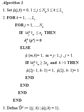
The set Ɗ̃ⁿ plays the role of flag, i.e., if the index (j,k) belongs to Ɗ̃ⁿ, then the numerical flux corresponding to the position (2j-1, k-1) is computed using a standard numerical scheme (in this paper, the characteristic-wise WENO scheme); otherwise, the flux is interpolated from coarser grids. This is a crucial point because, in general, computational cost to approximate numerical solution of hyperbolic conservation laws is concentrated on calculating numerical fluxes, particularly when a characteristic based scheme is employed.

The efficiency (15) of the multiresolution algorithm is measured by the ratio.

Numerical schemes

The equation (1) will be approximated by a semidiscrete conservative scheme, as the equation (16) indicates.

ρ_j(t) denotes the numerical approximation of ρ(x_j,t), h is the size of cell with center x_j and f_j+1/2 are the numerical fluxes.

The right hand side of equation (16) corresponds to an approximation of the spatial derivative ∂_x f(ρ) and it will be denoted by L_j (ρ(t)). In order to compute f_j+1/2 , the widely used fifth order WENO scheme (WENO-5) [11] is used. Due to nonlinearity of the model, it is necessary to split the flux into positive and negative parts, that is, f(ρ) = f⁺(ρ)+ f ^- (ρ). In this paper we employ the Lax-Friedrichs flux splitting f ^± (ρ) ∶=1/2 (f(ρ)±αρ). Here, the viscosity coefficient (or maximal characteristic velocity) α is estimated by the equation (17):

In order to implement a spectral version of WENO-5, the complete eigenstructure of J_f (ρ_j+1/2) are needed, that is, the normalized left eigenvectors I_j+1/2,i and the right eigenvectors r_j+1/2,i , i = 1, …, M of Jacobian matrix (the subscript j+1/2,i indicates the i-th eigenvector at the interface j+1/2). This information is provided by lemma 1.

Let R_j+1/2 be the matrix which columns are the right eigenvectors, thus the rows of its inverse matrix R^-1_j+1/2 are the left eigenvectors. With this information, it is possible to compute the local characteristic fluxes around the interface x_j+1/2 as the equation (18) shows:

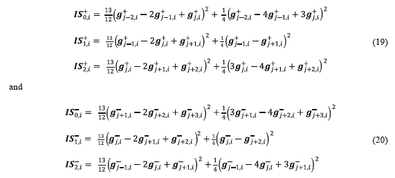
These fluxes are used to construct the smoothness indicators IS_p⁺ + and IS_p^- for p=0,1,2, which are given by the equations (19) and (20), respectively:

Next, the smoothness indicators are used to compute the weights ω_p⁺ + and ω_p^- for =0,1,2 . These weights are calculated by using the equations (21) and (22):

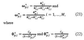
Here, the second subscript i denotes each characteristic field and the coefficients C_p for p=0,1,2, are the ideal weights [12] which are given by C_o=1/10, C₁=6/10 and C₂=3/10. The parameter δ>0 was originally introduced to avoid null denominator. However, as it is pointed out in [13], large values of δ may cause oscillations, while small values of δ may cause an order drop. In this paper, this parameter is taken as δ=10^-6, since this value is recommended in the literature [13].

Next, the equations (23) and (24) give the components of the characteristic numerical fluxes ĝ ⁺_j+1/2 and ĝ ^-_j+1/2 which are obtained by using the weights (24).

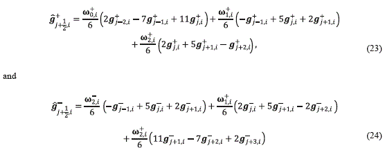
Next, it is necessary to perform the reconstruction in the physical space by the reverse projection as the equation (25) shows:

Finally, the numerical flux is formed by taking

In [1], the authors developed numerical simulation for the MCLWR model using adaptive multiresolution WENO schemes. However, they did not include spectral information, that is, the flux was computed in a component-wise manner.To solve the equation (16) maintaining high order in time with low storage requirements, we use an explicit strong-stability preserving time discretization method [14], in particular the optimal third-order, three-stage Runge-Kutta method, which is summarize in the equation (27):

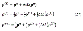
where the input ρⁿ approximates the solution at t=tⁿ=nΔt.

In order for the CFL (Courant-Friedrichs-Lewy) condition to be satisfied, the time step Δt is computed adaptively by , where σ is the Courant number and γⁿ_max is an estimation of the maximal characteristic velocity for ρⁿ. We recall that the CFL condition is a necessary condition for stability of the finite difference method (see [15] for more details) and numerical experience [16] suggests to take σ ≤ 0.6. In this work, we use σ = 0.2

Finally, we summarize the adaptive multiresolution spectral WENO scheme in the following algorithm. Given the solution ρ^n,0 on the finest grid at t = nΔt, the solution ρ^n+1,0 on the finest grid at t=(n+1)Δt is calculated by the following steps:

Algorithm 2

1. Calculate the set of significant points Ɗ̃ⁿ (see Algorithm 1)

2. Construct the multiresolution representation of and then, after discarding insignificant ρ^n,0 details recover the solution on the finest grid, this solution is denoted by ρ̃^n,0

3. Set ρ_jⁿ←ρ̃_j^n,0 for j=1,…,N_o, and use the Runge- Kutta method (29) to compute ρ_jⁿ⁺¹. At each Runge-Kutta stage, the operator L_j(∙) is computed from the numerical fluxes for all levels: using spectral WENO-5 if (j,k)∈ Ɗ̃ⁿ, otherwise Lagrange interpolation is used.

This procedure is repeated up to obtaining the numerical solution at the desired time.

Numerical experiments

This study considers a standard example from [2, 5, 17], with M=9 different classes of vehicles characterized by the maximum velocities v_i^max= (52.5+7.5i), i=1,…,9. The Drake's relationship (28) is used as the function V(ρ).

where the common parameter for all user classes ρ* is taken as 50veh/km. The initial condition (29) represent a platoon of maximum global density ρ=120veh/Km on highway 2 Km long.

Here, ρ(x) is the function given by equation (30)

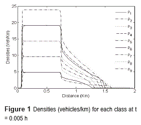
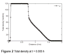
In figure 1, the profile of numerical solutions of each class is shown at t=0.005 h. Here, the tolerance considered is ε=10^-3 and three levels, i.e., L_c=3 and a finest grid with N₀=2⁸ points. The total density at the same time can be observed in figure 2. Notice the absence of oscillations close to discontinuities thanks the use of characteristic information.

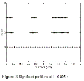
Figure 3 shows the positions of the significant points (elements that belong to Ɗ̃ⁿ) at each level. Notice that in zones where the solutions are smooth, significant positions at finest levels 1 and 2 do not appear, which means that in these zones flux evaluations are computed by interpolation. On the contrary, concentrations of elements of Ɗ̃ⁿ around shocks are observed. This shows the adaptive capabilities of multiresolution schemes to concentrate computational efforts in regions where it is actually necessary.

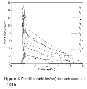
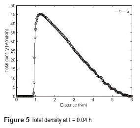
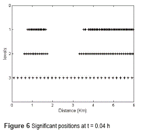
Figure 4 presents the evolution of the same problem at t=0.04h with its corresponding total densities (figure 5). The behavior of the significant positions is shown in figure 6. In [1] (see example 2) some oscillations are observed at the beginning of the road. We conjecture that such behavior is due to the implementation of WENO scheme in a component-wise manner.

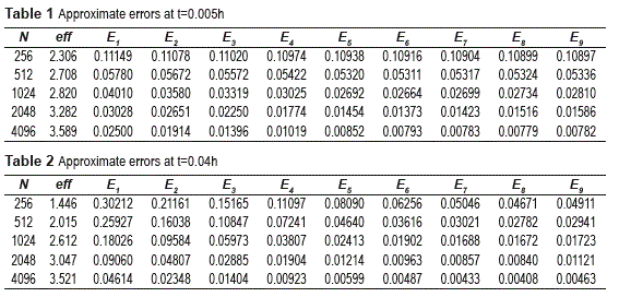
Tables 1 and 2 show the efficiency and the L¹ relative errors E_i ,i=1,…,M for each species. The errors are calculated according to the equation (31):

where ρ_i^N is the numerical solution for the i-th species with N∈{256,512,1024,2048,4096} and ρ_i^ref is a reference solution (exact solutions are not available) for the i-th species.

Conclusions

In this paper, adaptive multiresolution strategy is combined with a high order shock capturing method in order to design a robust code for numerical simulation of the multiclass Lighthill-Whitham-Richards traffic model. The novelty is that characteristic information is included for computing numerical fluxes. We provided numerical evidence of the advantage of multiresolution approach in order to obtain data compression, which implies computational savings.

We point out that the hyperbolicity analysis and subsequent characteristic structure obtained from lemma 1 is valid for rank-η perturbation of a diagonal matrix [18-20] with η≪M. Thus numerical approach considered in this work can be employed to other kinematic flow models.

Recently, in reference [21] the MCLWR model has been extended incorporating a diffusively corrected term, which takes into account anticipation lengths and reaction times. However, numerical simulations are developed with a second order scheme. The high order WENO method with multiresolution is a potential alternative in this case.

Acknowledgements

References

1. R. Bürger, A. Kozakevicius. ''Adaptive multiresolution WENO schemes for multispecies kinematic flow models''. J. Comput. Phys. Vol. 224. 2007. pp. 1190- 1222.         [ Links ]

2. R. Donat, P. Mulet. ''Characteristic-based schemes for multi-class Lighthill-Whitham-Richards traffic models''. J. Sci. Comput. Vol. 37. 2008. pp. 233-250.         [ Links ]

3. A. Harten. ''Multiresolution algorithms for the numerical solution of hyperbolic conservation laws''. Comm. Pure Appl. Math. Vol. 48. 1995. pp. 1305- 1342.         [ Links ]

4. S. Benzoni, R. Colombo. ''An n-populations model for traffic flow''. Eur. J. Appl. Math. Vol. 14. 2003. pp. 587-612.         [ Links ]

5. G. Wong, S. Wong. ''A multi-class traffic flow model - an extension of LWR model with heterogeneous drivers''. Transp. Res. A. Vol. 36. 2002. pp. 827-841.         [ Links ]

6. P. Zhang, R. Liu, S. Wong, S. Dai. ''Hyperbolicity and kinematic waves of a class of multi-population partial differential equations''. Eur. J. Appl. Math. Vol. 17. 2006. pp. 171-200.         [ Links ]

7. R. Donat, P. Mulet. ''A secular equation for the Jacobian matrix of certain multispecies kinematic flow models''. Numer. Methods Partial Differential Equations. Vol. 26. 2010. pp. 159-175.         [ Links ]

8. R. Bürger, A. Kozakevicius, M. Sepúlveda. ''Multiresolution schemes for strongly degenerate parabolic equation in one space dimension''. Numer. Meth. Partial Diff. Eqns. Vol. 23. 2007. pp. 706-730.         [ Links ]

9. A. Cohen, S. Kaber, S. Müller, M. Postel. ''Fully adaptive multiresolution finite volume schemes for conservation laws''. Math. Comp. Vol. 88. 2001. pp. 399-443.         [ Links ]

10. A. Harten. ''Multiresolution representation of data: a general framework''. SIAM J. Numer. Anal. Vol. 33. 1996. pp. 1205-1256.         [ Links ]

11. C. Shu. ''Essentially non-oscillatory and weighted essentially non-oscillatory schemes for hyperbolic conservation laws''. B. Cockburn, C. Johnson, C. W. Shu, E. Tadmor (editors). Advanced Numerical Approximation of Nonlinear Hyperbolic Equations. Ed. Springer-Verlag. Berlin, Germany. 1998. pp. 325- 432.         [ Links ]

12. G. Jiang, C. Shu. ''Efficient implementation of weighted ENO schemes''. Journal of Computational Physics. Vol. 126. 1996. pp. 202-228.         [ Links ]

13. A. Henrick, T. Aslam, J. Powers. ''Mapped weighted essentially non-oscillatory schemes: Achieving optimal order near critical points''. J. Comput. Phys. Vol. 207. 2005. pp. 542-567.         [ Links ]        [ Links ]

15. R. Le Veque. Finite Volume Methods for Hyperbolic Problems. 1^st ed. Ed. Cambridge University Press. Cambridge, UK. 2002. pp. 68.         [ Links ]

16. P. Zhang, S. Wong, S. Dai. ''A note on the weigthed essentially non-oscillatory numerical scheme for a multi-class Lighthill-Whitham-Richards traffic flow model''. Commun. Numer. Meth. Engng. Vol. 25. 2009. pp. 1120-1126.         [ Links ]

17. M. Zhang, C. Shu, G. Wong, S. Wong. ''A weighted essentially non-oscillatory numerical scheme for a multi-class Lighthill-Whitham-Richards traffic flow model''. J. Comput. Phys. Vol. 191. 2003. pp. 639-659.         [ Links ]

18. J. Anderson. ''A secular equation for the eigenvalues of a diagonal matrix perturbation''. Lin. Alg. Appl. Vol. 246. 1996. pp. 49-70.         [ Links ]

19. R. Bürger, R. Donat, P. Mulet, C. Vega. ''Hyperbolicity analysis of polydisperse sedimentation models via a secular equation for the flux Jacobian''. SIAM J. Appl. Math. Vol. 70. 2010. pp. 2186-2213.         [ Links ]

20. R. Bürger, R. Donat, P. Mulet, C. Vega. ''On the implementation of WENO schemes for a class of polydisperse sedimentation models''. J. Comput. Phys. Vol. 230. 2011. pp. 2322-2344.         [ Links ]

21. R. Bürger, P. Mulet, L. Villada. ''A diffusively Corrected Multiclass Lighthill-Whitham-Richards Traffic Model with Anticipation Lengths and Reaction Times''. Adv. Appl. Math. Mech. Vol. 5. 2013. pp. 728- 758.         [ Links ]