ARTÍCULO ORIGINAL

DOI: 10.17533/udea.redin.n77a09

Drought and genetic programming to approach annual agriculture production normalized curves

Sequía y programación genética para aproximar curvas normalizadas de producción agrícola anual

Ariadne Sofía Drust-Nacarino¹, Maritza Liliana Arganis-Juaréz^1,2*, Rodolfo Silva-Casarín¹, Edgar Gerardo Mendoza -Baldwin¹, Óscar Arturo Fuentes-Mariles²

¹Instituto de Ingeniería, Universidad Nacional Autónoma de México. Ciudad Universitaria. C. P. 04510. México, D. F., México.

²Facultad de Ingeniería, Universidad Nacional Autónoma de México. Ciudad Universitaria. C. P. 04510. México, D. F., México.

* Corresponding author: Maritza Liliana Arganis Juárez, e-mail: marganisj@iingen.unam.mx 

(Received February 23, 2015; accepted May 11, 2015)

ABSTRACT

Drought is a severe, recurrent disaster for Mexican agriculture, causing huge economic losses, which could be reduced if appropriate planning and policies were carried out and the production loss could be predicted. This paper presents the application of a genetic programming scheme to obtain normalized curves of annual agricultural production for each state in Mexico as a function of the return period of drought events and, from them, compute the normalized value of the yearly production. This value, multiplied by the historic mean production of the state, gives the production expressed in Mexican pesos for a specified return period. Two techniques were used for this data analysis, the first one is general and considers each state separately; for the second technique the country was divided into six groups, depending on the value of the agricultural production variation coefficient. The results showed that for the first case large dispersion was found between the reported and computed data, while a better fit was found for the groups; specifically for groups 2, 3 and 6. The resulting functions can be used by decision makers at both federal and state levels, to better deal with drought events.

Keywords: Drought, genetic programming, agricultural production, regionalization, economic loss

RESUMEN

La sequía es un severo desastre, recurrente para la agricultura mexicana, que causa enormes pérdidas económicas que podrían reducirse si se contara con políticas y planeación adecuadas y se pudiera predecir la reducción en la producción ante su ocurrencia. En este estudio se presenta la aplicación de un esquema de programación genética para obtener curvas normalizadas de producción agrícola anual para cada estado de la República Mexicana en función del periodo de retorno de eventos de sequías y, a partir de ellas, estimar el valor normalizado de la producción anual. Este valor al ser multiplicado por la media histórica de la producción en el estado, proporciona la producción expresada en pesos mexicanos para un periodo de retorno específico. Dos técnicas fueron utilizadas para este análisis de datos, la primera es general e incluye cada estado por separado; en la segunda técnica el país fue dividido en seis grupos, dependiendo del valor del coeficiente de variación de la producción agrícola. Los resultados mostraron que en el primer caso se tiene una gran dispersión entre los datos medidos y calculados, mientras que se halló un mejor ajuste cuando se utilizaron grupos; especialmente en los grupos 2, 3 y 6. Las funciones encontradas pueden utilizarse por los tomadores de decisiones tanto a nivel estatal como a nivel federal, para abordar los eventos de sequía.

Palabras clave: Sequía, programación genética, producción agrícola, regionalización, pérdidas económicas

1. Introduction

In recent years, large-scale intensive droughts have been observed worldwide [1, 2] leading to high economic and social costs [3]. In North America, the impact of the 1988 drought on the US economy has been estimated in 40 billion USD [4]. Based on the available data from the National Climatic Data Center, nearly 10 % of the total land area of the United States experienced either severe or extreme droughts at any given time during the last century. From 1980 to 2003, in the United States as a whole, droughts accounted for 10 of the 58 weather-related disasters and accounted for 144 billion USD, i.e. 41.2 % of the national cost of these disasters [4].

In Europe, there was a prolonged drought over large areas associated with the summer heat wave of 2003 [5]. In the Iberian Peninsula the most serious drought in 60 years occurred in 2005, reducing overall EU cereal yields [6]. In Asia, according to a recent IPCC study, production of rice, corn and wheat has declined due to increasing water stress, arising partly from increasing temperature, increasing frequency of El Niño events and a reduction in the number of rainy days [7]; India is amongst the most vulnerable drought-prone countries in the world [8]. The Australian Bureau of Agriculture and Resource Economics estimates that the 2006 drought reduced the national winter cereal crop by 36 % and cost rural Australia around 3.5 billion AUD, leaving many farmers in financial crisis [9]. In Africa, droughts have had a devastating impact on this ecologically vulnerable region and were a major impetus for the establishment of the United Nations Convention on Combating Desertification and Drought [6].

Recently, extreme droughts in Mexico and their consequent water deficits have become more frequent, causing serious problems to the economy of the nation. The regions which are most severely affected by drought in Mexico are the north, northwest and northeast, where 90 % of the irrigation zones and 70 % of the industrial plants are located [10]. These areas have high demand for water, yet receive less than 40 % of the national rainfall; furthermore, agriculture consumes more than 85 % of the water available [10]. An important characteristic of droughts in Mexico is their spatial distribution: in general, they affect large areas, and local response contributes little to solve the overall problem and while some areas are only slightly affected, other places suffer severe impact [10]. In Mexico many studies have focused on the meteorological aspects of drought [11, 12], defined as a function of the rainfall deficit (expressed as the ratio of the average annual rainfall and its duration in a given geographical region) and on the prediction of which areas of the country are most vulnerable to this phenomenon.

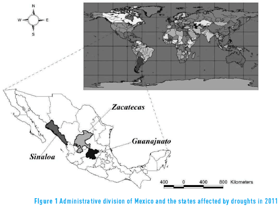
Mexico is located mainly in North America and partially in Central America. The continental area is 1.9 million square kilometres, with 5127 square kilometres of insular surface Mexico is located mainly in North America and partially in Central America. The continental area is 1.9 million square kilometres, with 5127 square kilometres of insular surface. The territory is divided into 31 states and one Federal District (Figure 1) [13]. A large part of Mexico is in the strip of northern latitude, high pressure, with arid and semi-arid areas; coinciding in latitude with African, Asian and Australian deserts [14]. This means that, geographically, Mexico is located in a region prone to drought events especially in the regions where rainfall has historically been lower.

The most important investigations from a historical point of view, have been made by social scientists such as [15, 16] who was interested in the droughts in the Valley of Mexico and the Bishopric of Michoacán (1708-1810), [17] studied the droughts of the nineteenth century. [18, 19] highlighted the importance of drought at a national level as one of the main causes of the agricultural crises of the past.

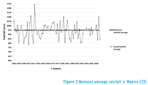
The ecophysiological response to drought and recovery after rainfall were evaluated for three endemic tree species [20]. [21] studied a group of 'Flor de Mayo' dry bean cultivars regarding their response to drought, high temperatures and breeding advances. In 2013 [14] based her research in San Juan Guelavia, Oaxaca, examining how some of Mexico's two million small farmers are responding to the opening of the market for corn; her research largely examines how the liberalization of corn between the US and Mexico and local responses to faltering corn production and markets have reconfigured the physical, social, political, historical, and economic landscape of indigenous maize farming communities in southern Mexico [14]. In 2010, the national annual mean rainfall value was 17.5 % higher than the period 1981-2010 average (935.7 mm), while in 1982, 1988, 1995, 1996, 2009 and 2011 it was under this average (Figure 2) [22].

Extraordinary drought events occurred in 1957, 1969, 1982, 1997 and 2011. The recent drought in 2011 primarily affected northern Mexico but global warming–associated climate change is projected to cause drying of the whole country. If the base climatology of Mexico is changing, the most vulnerable region may actually be the 13 states of Central Mexico which have 40 % of Mexican territory and nearly 75 million inhabitants [24]. This region has the highest population density in Mexico and includes Mexico City, the city with the highest national water demand and where the regional aquifers and watersheds are already being depleted [25]. Although warming here may lengthen the growing season [26], ''the projected drying of this region both in winter, by an intensified atmospheric moisture divergence and a poleward expanded subtropical dry zone, and in summer, by a weaker Mexican monsoon, will add further stress to water resources and could lead to ecological change and negative impacts on agriculture and economic instability'' [27].

Drought affects a large number of states and in agricultural production, the differences between the sown and harvested areas are evident; exports decrease and there are monetary losses. There is always somewhere in the northern part of Mexico suffering from a drought. Weather reports indicate that three of every five years are dry and that droughts can be seasonal, annual or multi-annual. The financial losses of the 2011 drought surpassed 16 billion Mexican pesos (1.3 billion USD) including losses of 9 billion Mexican pesos (710 million USD) for corn and 6 billion Mexican pesos (280 million USD) for beans [28]. The Secretariat of Agriculture, Livestock, Rural Development, Fisheries and Food [29] said that in the agricultural year of 2011, 2.7 million hectares of land were affected in seven of the main crops, especially in Sinaloa, Zacatecas, and Guanajuato (Figure 1).

This study deals with obtaining normalized equations, which can forecast the annual agricultural production in Mexico as a function of drought with a certain return period. Genetic programming was considered for this purpose.

For this study the data processed was obtained from the SIAP (Servicio de Información Agroalimentaria y Pesquera) for the period 2003-2011, taking the agricultural production values in Mexico [30] and the annual averages of droughts reported by CONAGUA (National Committee of Water) for the same period, to obtain a function of the data and generate an equation through the application of genetic programming.

2. Methods

2.1. Genetic programming

Genetic programming is an algorithm of evolutionary computing which allows the generation of mathematical models by means of operations similar to those applied in genetic algorithms [2, 31, 32]. In this case the individuals are sets of operators, constants and variables which are selected, crossed and even mutated (that is to change from one operator to another or to one variable to another) in order to get a final model which satisfies an objective function. Genetic programming has been recently applied in many engineering works: [1] performed wave predictions by applying genetic programming, [24] used genetic programming to develop a universal equilibrium predictor for ripple wavelength, height, and steepness, [33] applied genetic programming in estimating saturated hydraulic conductivity, [34] used linear genetic programming to predict flow discharge in compound channels and [35] used the genetic programming to forecast the wave heights with lead times of 12 h and 24 h.

This study aims to obtain normalized curves of annual agricultural production in Mexico depending on the return period of a drought event; the genetic programming algorithm [36, 37] is a sub-class of the well-known genetic algorithm. It involves the random generation of an initial population of trees, constituted by a set of functions and variables relevant to the problem to be solved, defining the objective function to evaluate the fitness of each defined function. Then, as in the case of traditional genetic algorithms, the best fit functions are selected and subjected to the operators of crossover, mutation and reproduction in order to generate a new population of models, representing the next generation.

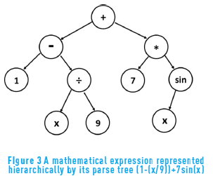
A typical genetic programming algorithm (GP) consists of a set of functions, which can involve arithmetic operators (+,−,∗, /, . . .), transcendental functions (sin, cos, tan,. . . , ln, exp,. . . ), even relational operators (>, <,=) or conditional operators (IF), and a terminal set with variables and constants (x₁, x₂, x₃, . . . x_n). An initial population is randomly created with a number of parse tree individuals composed of nodes (operators plus variables and constants), previously defined according to the problem domain. An example of a GP individual is given in Figure 3.

An objective function must be defined to evaluate the fitness of each individual (in this case each individual will be a resultant model or program of the random combination of nodes). Selection, crossover, and mutation operators are then applied to the best individuals, and a new population is created. The whole process is repeated until the given generation number is reached [2].

In this research both arithmetic and transcendental operators were taken into account; so the terminal set vector TS was: Ts= [+,-,*/, exp, sin, cos]; the variable y (normalized data of production in millions of pesos) and the independent variable x (return period in years, of the normalized data). The maximum number of nodes considered were 15, 400 individuals, a cross probability of 0.9, a mutation probability of 0.05 with 10000 generations used.

The objective function was to minimize the mean square error between the measured data and that calculated by the genetic programming model.

2.2. Regionalization

This is the process used for taking several samples, forming a new sample, representative of the entire region, with the largest number of data, from which the most reliable statistics are obtained and which can then be applied in each site in the region.

The regionalization process is made up by the following steps: 1) Using functions of transformation in order to preserve the common statistical characteristics (similar variation coefficient), eliminating the effect of dispersion from the individual different characteristics (the mean or the standard deviation only) so as to achieve a homogeneous data sample. 2) Using statistics, such as Fisher's exact test, the functions of most appropriate transformation are selected and those with distinctive characteristics that could not be eliminated by any transform function are deleted.

The homogeneous sample is fitted to a probability distribution function and the magnitude of the transformed values for different return periods is estimated.

2.3. Data set

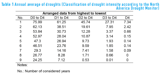
With monthly percentages taken from the CONAGUA web site [38], annual averages of drought at national level were calculated for the period 2003-2011. The data was then ordered from highest to lowest as shown in Table 1.

Abnormally dry (D0): this is a condition of dryness; it is not a category of drought. It occurs at the beginning or end of a period of drought. At the beginning of a period of drought, if short-term, it can cause delay in the planting of crops, a limited growth of crops or pastures and there is a risk of fire. At the end of the period of drought a water deficit may persist and pastures or crops may not fully recover.

Moderate drought (D1): produces some damage to crops and pastures; there is a high risk of fire, low levels in rivers, streams, reservoirs, water troughs and wells. Voluntary restraint in the use of water is suggested.

Severe drought (D2): causes probable losses in crops or pastures, high risk of fire, water scarcity is common. Restrictions on the use of the water must be imposed.

Extreme drought (D3): greater losses in crops and pastures, the risk of forest fires is extreme. Sweeping restrictions on the use of water are necessary.

Exceptional drought (D4): exceptional, widespread losses of crops or pastures, exceptional risk of fires, total shortage of water in reservoirs, streams and wells. An emergency situation is likely due to the absence of water.

3. Discussion and results

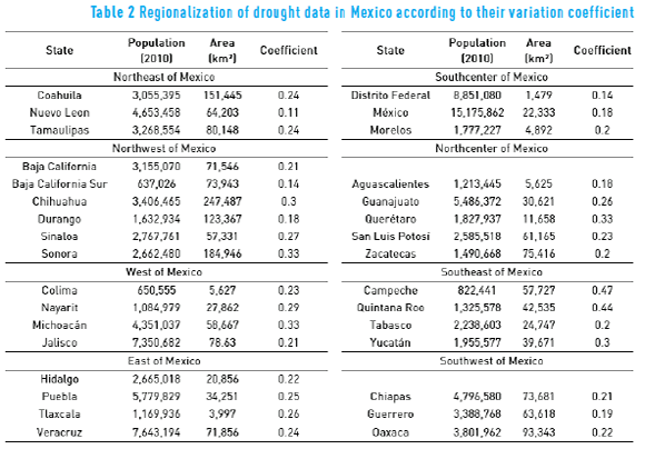
The D3 to D4 droughts for Mexico from 2003-2011 were regionalized, according to their variation coefficients, as shown in Table 2.

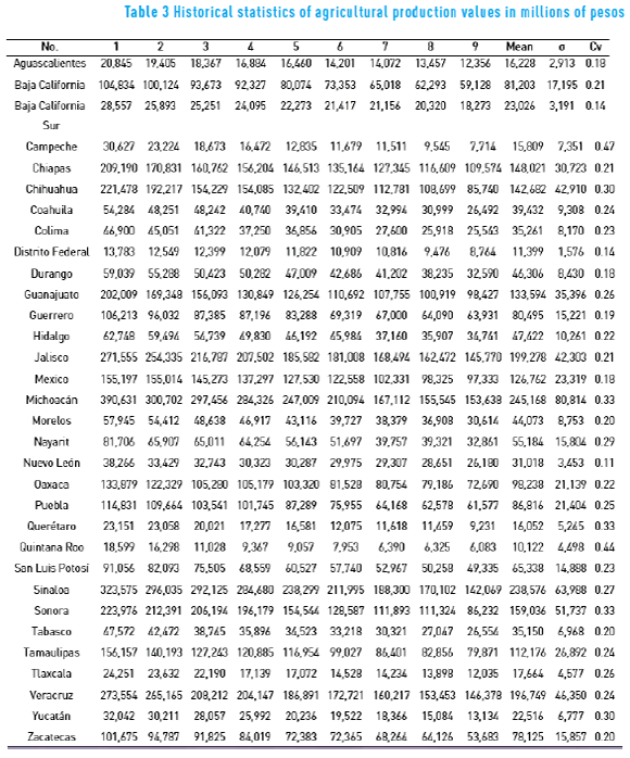
The agricultural production value of the crop data, in thousand millions of pesos, for the period 2003-2011, was obtained from SIAP, with data arranged from the highest to the lowest value for each region, as indicated by the numbers 1-9 in Table 3. The mean, standard deviation (s_x) and variation coefficient (Cv) were calculated using the following Eqs. (1-3):

Mean:

Standard Deviation (Sd)

Variation coefficient

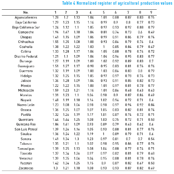
Then the data were normalized by dividing each production value in thousands of millions of pesos by their calculated mean, for example for Tlaxcala the greatest normalized data is: 2,425,149/1,776,442 =1.37, see Table 4.

For the first case a y = f (x)function was generated with GP; the value of x is the return period in years, obtained with the Weibull equation (n+1)/m, where n is the size of annual series, m is the number of the ordered data, and y represents the normalized data of the agricultural production. In this case only one register was built considering the data for all the states.

The result of the first case Eq. (4) is:

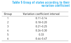
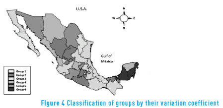
For the second case a set of y=f(x) functions were also generated, the x values are the same as case 1, but the values of y (normalized annual production) were divided into 6 groups of States Table 5, Figure 4), according to the following intervals of the variation coefficient obtained from Table 3.

The Eqs. (5-10) generated for each group of states are

Group 1:

Group 2:

Group 3:

Group4:

Group 5:

Group 6:

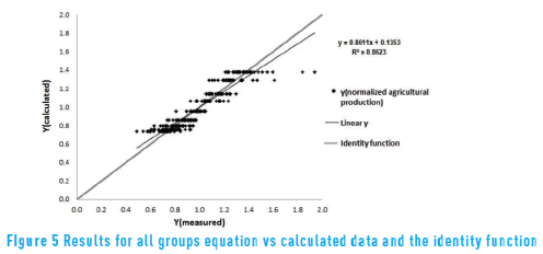
In Figure 5, the results obtained in Eq. (4) against the calculated data and versus the identity function with a determination coefficient of 0.8623 (i.e. a correlation coefficient of 0.9286) are shown.

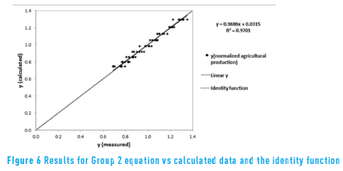
In Figure 6, the comparison between the results given by the Group 2 equation against the calculated data and versus the identity function, with a determination coefficient of 0.9701 (that is a correlation coefficient of 0.9849) is presented.

Table 6 shows the determination and correlation coefficients obtained with Eqs. (4) and (6).

Several studies on the calculation of return periods of drought severity can be found e.g. [39-41]. This means that an engineer or a decision maker can know the return period for a specific drought; using one of these models. It is possible to estimate the agricultural production due to a specific drought event in a federal analysis or in a State analysis.

It is important to consider the short period of historical data available. The return period was obtained only as a function of the number or order; and the models must be applied to interpolate data, and extrapolations are suggested for return periods near to 10 years.

If the recorded data has not enough information about the climate change it is not possible to evaluate it. Nevertheless, in case of availability, the climate variability must be analyzed in a different way (see [42]). Currently there is much discussion about how climatology is changing [43].

New models can be obtained according to new data recorded year after year, to take into account the variability in the climate.

3.1. Example of the application of the obtained equations

To better explain the equations used in this work, the data recorded for Zacatecas is given in Tables 7 and 8, where the normalized historical agricultural production for a return period of 10 years and the calculated values obtained with Eqs. (4) and (6) are shown.

If Zacatecas has a drought with a return period of 10 years, the expected production y (normalized) would be 1.377. If, historically, the average production has been of 7.812 billion pesos, then the expected production will be the result of Eq. (4) multiplied by the average historical production that is (1.377) (7.812) = 10.757 billion pesos.

When a local group analysis is carried out by decision makers, the results can be slightly different. For example if Eq. (6) is applied to group 2, where Zacatecas belongs, in that return period, 1.2961 of the normalized production times the average gives (1.2961)(7.812)= 10.125 billion pesos.

In Table 9 it is seen that the differences obtained in the expected agricultural production when analysis is made for the whole country (federal level) are greater than those for the analysis made for state level.

4. Conclusions

Annual agricultural production normalized curves as a function of the return period for droughts D3 and D4, obtained with genetic programming, using all normalized data, give a clear idea about the expected value of production if such a drought takes place. The normalization of annual agricultural production data according to their variation coefficient allowed us to identify regions with similar behaviour and a new set of equations were determined with genetic programming for each group. Such equations can be applied for short term forecasting purposes in economic planning before a drought event at state and federal levels.

Drought events in Mexico are traditionally solved with corrective measures once losses in agriculture and livestock farming have occurred. The determination of models that allow predictions of production before a drought is considered a useful practical tool for making important decisions in the country by the authorities in charge.

The applied methodology can be applied to longer recorded data and is independent from the type of the variables, so it is possible to get models involving agriculture production against floods, rainfall or another data related to natural disasters.

5. References

1. A. Kambekar and M. Deo, ''Wave prediction using genetic programming and model trees'', Journal of Coastal Research, vol. 28, pp. 43-50, 2012.         [ Links ]

2. J. Koza, ''Hierarchical genetic algorithms operating on populations of computer programs'', in 11^th International Joint Conference on Artificial Intelligence, Detroit, USA, 1989, pp. 768-774.         [ Links ]

3. C. Escalante and L. Reyes, ''Análisis de la sequía meteorológica en el norte de México'', in XXII National Congress of Hydraulic, Acapulco, México, 2012, pp. 1-8.         [ Links ]

4. T. Ross and N. Lott, ''A climatology of 1980–2003 extreme Weather and climate events'', National Climatic Data Center, Asheville, USA, Tech. Rep. 2003-01, Dec. 2003.         [ Links ]

5. L. Feyen and R. Dankers, ''Impact of global warming on streamflow drought in Europe'', Journal of geographical Research-Atmospheres, vol. 114, pp. 1-17, 2009.         [ Links ]

6. N. Zeng, ''Drought in the Sahel'', Science, vol. 302, pp. 999-1000, 2003.         [ Links ]

7. B. Bates, Z. Kundzewicz, S. Wu and J. Palutikof, ''Climate change and water'', Intergovernmental Panel on Climate Change (IPCC), Geneva, Switzerland, Tech. Paper VI. Jun. 2008.         [ Links ]

8. Food and Agricultural Organisation of United Nations (FAO), ''Report of FAO-CRIDA Expert Group Consultation on Farming System and Best Practices for Drought-prone Areas of Asia and the Pacific Region'', Central Research Institute for Dryland Agriculture, Hyderabad, India, Report, 2002.         [ Links ]

9. G. Wong, M. Lambert and A. Metcalfe, ''Trivariate copulas for characterisation of droughts'', ANZIAM, vol. 49, pp. 306-323, 2008.         [ Links ]

10. C. Escalante, ''La vulnerabilidad ante los extremos: la sequía'', Ingeniería Hidráulica en México, vol. 18, pp. 133-155, 2003.         [ Links ]

11. G. Garza, ''Climatología histórica: las ciudades mexicanas antes de la sequía (siglos XVII a XIX)'', Investigaciones Geográficas, vol. 63, pp. 77-92, 2007.         [ Links ]

12. I. Flores and D. Campos, ''Detección de periodos de sequía en la zona media del estado de San Luis Potosí, con base en registros precipitación mensual'', Ingeniería Hidráulica en México, vol. 13, pp. 45-56, 1998.         [ Links ]

13. INEGI (National Institute of Statistics and Geography), Referencias geográficas y extensión territorial de México. [Online]. Available: http://www.inegi.org.mx/inegi/SPC/doc/internet/1-GeografiaDeMexico/MAN_REFGEOG_EXTTERR_VS_ENERO_30_2088.pdf. Accessed on: Jun. 1, 2015.         [ Links ]

14. A. Browning, ''Corn, tomatoes, and a dead dog: Mexican agricultural restructuring after NAFTA and rural responses to declining maize production in Oaxaca, Mexico'', Mexican Studies, vol. 29, pp. 85-119, 2013.         [ Links ]

15. E. Florescano and L. Espinosa, Fuentes para el estudio de la agricultura colonial en la diócesis de Michoacán. Series de diezmos, 1636-1810, 1st ed. México, D. F., México: Instituto Nacional de Antropología e Historia, 1987.         [ Links ]

16. E. Florescano and S. Swan, Breve historia de la sequía en México, 1^st ed. Xalapa, México: Universidad Veracruzana, Dirección Editorial, 1995.         [ Links ]

17. G. Castorena, E. Sánchez, E. Florescano, G. Padilla and L. Rodríguez, Análisis histórico de las sequías en México. México, D. F., México: Secretaría de Agricultura y Recursos Hidráulicos, 1980.         [ Links ]

18. D. Comte, ''Weather highlights around the world'', Weatherwise, vol. 47, pp. 23-26, 1994.         [ Links ]

19. D. Comte, ''Weather highlights around the world'', Weatherwise, vol. 48, pp. 20-22, 1995.         [ Links ]

20. J. Martínez and A. Fernández, Cambio climático: una visión desde México, 1^st ed. México, D. F., México: Instituto Nacional de Ecología, 2004.         [ Links ]

21. E. Barrios et al., ''Avances en el mejoramiento genético del frijol en México por tolerancia a temperatura alta y a sequía'', Revista Fitotecnia Mexicana, vol. 34, pp. 247-255, 2011.         [ Links ]

22. E. Pimienta, C. Robles and C. Martínez, ''Respuesta ecofisiológica de árboles jóvenes nativos y exóticos a sequía y lluvia'', Revista Fitotecnia Mexicana, vol. 35, pp. 15-20, 2012.         [ Links ]

23. Secretaría de Medio Ambiente y Recursos Naturales (SEMARNAT), ''Informe de la situación del medio ambiente en México. Compendio de estadísticas ambientales indicadores clave y de desempeño ambiental'', SEMARNAT, México, D. F., México, Report, 2013.         [ Links ]

24. E. Goldstein, G. Coco and A. Murray, ''Prediction of wave ripple characteristics using genetic programming'', Continental Shelf Research, vol. 71, pp. 1-15, 2013.         [ Links ]

25. Comisión Nacional del Agua, Estadísticas del agua en México. Sistema Nacional de Información sobre Cantidad, Calidad, Usos y Conservación del Agua. México, D. F., México: Comisión Nacional del Agua, 2006.         [ Links ]

26. C. Conde, R. Ferrer and S. Orozco, ''Climate change and climate variability impacts on rain–fed agricultural activities and possible adaptation measures. A mexican case study'', Atmósfera, vol. 19, pp. 181-194, 2006.         [ Links ]

27. G. Medina, C. Ruiz and P. Martínez, Los Climas de México: Una Estratificación Ambiental Basada en el Componente Climático. Guadalajara, México: Centro de Investigación Regional del Pacífico Centro, INIFAP, SAGAR, 1998.         [ Links ]

28. M. Hernandez, L. Torres and G. Valdez, ''Sequía meteorológica'', in México: una visión hacia el siglo XXI. El cambio climático en México, C. Gay (ed). México, D. F., México: Instituto Nacional de Ecología, SEMARNAP, Universidad Nacional Autónoma de México, U.S. Country Studies Program, 2000, pp. 25-40.         [ Links ]

29. SAGARPA, Secretaría de agricultura, ganadería, desarrollo rural, pesca y alimentación, 2015. [Online]. Available: http://www.sagarpa.gob.mx/Paginas/default.aspx. Accessed on: Jun. 1, 2015.         [ Links ]

30. W. Riebsame and A. Magalhaes, ''Assessing the regional implications of climate variability and change'', in 2^nd World Climate Conference, Geneva, Switzerland, 1990, pp. 415-430.         [ Links ]

31. N. Cramer, ''A representation for the adaptive generation of simple sequential programs'', in 1^st International Conference on Genetic Algorithms and the Applications, Pittsburgh, USA, 1985, pp. 183-187.         [ Links ]

32. J. Koza, Genetic Programming. On the Programming of Computers by Means of Natural Selection, 1^st ed. Cambridge, USA: MIT Press, 1992.         [ Links ]

33. K. Parasuraman, A. Elshorbagy and C. Bing, ''Estimating Saturated Hydraulic Conductivity Using Genetic Programming'', Soil Science Society of American Journal, vol. 71, pp. 1676-1684, 2007.         [ Links ]

34. H. Azamathulla and A. Zahiri, ''Flow discharge prediction in compound channels using linear genetic programming'', Journal of Hydrology, vol. 454-455, pp. 203-207, 2012.         [ Links ]

35. S. Nitsure, S. Londhe and K. Khare, ''Wave forecasts using wind information and genetic programming'', Ocean Engineering, vol. 54, pp. 61-69, 2012.         [ Links ]

36. W. Banzhaf, P. Nordin, R. Keller and F. Francone, Genetic Programming: An Introduction: On the Automatic Evolution of Computer Programs and its Applications. San Francisco, USA: Morgan Kaufmann Publishers Inc., 1998.         [ Links ]

37. B. Juárez and E. Hansen, ''Mexico: Grain and Feed Annual. Prolonged Drought Devastates Grain and Feed Sector'', Global Agricultural Information Network, Rep. MX2018, Mar. 2012. [Online]. Available: http://gain.fas.usda.gov/Recent%20GAIN%20Publications/Grain%20and%20Feed%20Annual_Mexico%20City_Mexico_3-30-2012.pdf. Accessed on: Jun. 1, 2015.         [ Links ]

38. Comisión Nacional del Agua (CONAGUA), Resúmenes Mensuales (consulta de tabla nacional por entidad federativa y mapas), 2015. [Online]. Available: http://smn.cna.gob.mx/index.php?option=com_%20content&view= article& id= 12 &Itemid=77. Accessed on: Jun. 1, 2015.         [ Links ]

39. B. Bonaccorso, A. Cancelliere and G. Rossi, ''An analytical formulation of return period of drought severity'', Stochastic Environmental Research and Risk Assessment, vol. 17, pp. 157-174, 2003.         [ Links ]

40. N. Dalezios, A. Loukas, L. Vasiliades and E. Liakopoulos, ''Severity-duration-frequency analysis of droughts and wet periods in Greece'', Hydrological Sciences Journal, vol. 45, pp. 751-769, 2000.         [ Links ]

41. Z. Zhou and Z. Wang, ''Theory of Drought System Analysis'', Nature and Science, vol. 1, pp. 62-66, 2003.         [ Links ]

42. R. Katz and B. Brown, ''Extreme events in a changing climate: variability is more important than averages'', Climatic change, vol. 21, pp. 289-302, 1992.         [ Links ]

43. T. Knutson et al., ''Tropical cyclones and climate change'', Nature Geoscience, vol. 3, pp. 157-163, 2010.         [ Links ]