ARTÍCULO ORIGINAL

DOI: 10.17533/udea.redin.n79a11

Data envelopment analysis and Pareto genetic algorithm applied to robust design in multiresponse systems

Data envelopment analysis and Pareto genetic algorithm applied to robust design in multiresponse systems

Enrique Carlos Canessa-Terrazas¹*, Filadelfo de Mateo-Gómez^2, Wilfredo Fernando Yushimito Del Valle¹

¹Facultad de Ingeniería y Ciencias, Universidad Adolfo Ibáñez. Av. Padre Hurtado 750. C. P. 2520000. Viña del Mar, Chile.

²Escuela de Ingeniería Industrial, Facultad de Ingeniería, Universidad de Valparaíso. Av. Brasil 1786. C. P. 2340000. Valparaíso, Chile.

* Corresponding author: Enrique Carlos Canessa Terrazas, e-mail: ecanessa@uai.cl

DOI: 10.17533/udea.redin.n79a11

(Received March 30, 2015; accepted February 17, 2016)

ABSTRACT

This paper shows the use of Data Envelopment Analysis (DEA) to rank and select the solutions found by a Pareto Genetic Algorithm (PGA) to problems of robust design in multiresponse systems with many control and noise factors. The efficiency analysis of the solutions using DEA shows that the PGA finds a good approximation to the efficient frontier. Additionally, DEA is used to determine the combination of a given level of mean adjustment and variance in the responses of a system, so as to minimize the economic cost of achieving those two objectives. By linking that cost with other technical and/or economic considerations, the solution that best matches a predefined level of quality can be more sensibly selected.

Keywords: Robust design, Taguchi methods, Pareto genetic algorithms, data envelopment analysis

RESUMEN

Se presenta el uso de Análisis Envolvente de Datos (AED) para priorizar y seleccionar soluciones encontradas por un Algoritmo Genético de Pareto (AGP) a problemas de diseño robusto en sistemas multirespuesta con muchos factores de control y ruido. El análisis de eficiencia de las soluciones con AED muestra que el AGP encuentra una buena aproximación a la frontera eficiente. Además, se usa AED para determinar la combinación del nivel de ajuste de media y variación de las respuestas del sistema, y con la finalidad de minimizar el costo económico de alcanzar dichos objetivos. Al unir ese costo con otras consideraciones técnicas y/o económicas, la solución que mejor se ajuste con un nivel predeterminado de calidad puede ser seleccionada más apropiadamente.

Palabras clave: Diseño robusto, métodos Taguchi, algoritmo genético Pareto, análisis envolvente de datos

1. Introduction

Robust design is a technique developed by Genichi Taguchi that tries to enhance the quality of products and/or services by reducing the variability of the outputs of the service or manufacturing process and, simultaneously, adjusting the mean of the outputs as close as possible to their corresponding target values [1]. Generally, the procedure involves experimenting with controllable input variables of the system (control factors) under different settings of variables that increase the variability of outputs and/or move the outputs away from their target values (noise factors), and analyzing the output data to find combinations of values of control factors that achieve both objectives of robust design [2]. Although the technique can be straightforwardly applied to single response systems with a small number of control and noise factors, it becomes hard to use in multiresponse systems with many outputs, control, and noise factors [3-6]. Among the alternatives to overcome the complexity of multiresponse systems, it has been widely noticed that Genetic Algorithms (GA) [7, 8] are well-suited for robust design [4, 9] due to its ability to handle in parallel populations related to multiple solutions. One of the Genetic Algorithm models that handle multiresponse systems in robust design is a Pareto GA (PGA) developed in [10]. This PGA finds the efficient solutions, which attain the lowest possible variation of the outputs of the system, without degrading the mean adjustment of them and vice-versa. However, even selecting the best solution among the Pareto efficient ones will depend on a variety of considerations, i.e., the cost, time, and/or constraints of implementing each of them; or the relative influence of reducing variability and increasing mean adjustment on the quality of the service or product delivered to customers. As there are many trade-offs that can be considered, it is usually difficult to decide among the candidate solutions.

To help in that decision, this paper presents the use of Data Envelopment Analysis (DEA) [11] as a method for assessing the relative merit of each solution obtained by the PGA model. DEA is a nonparametric method of operations research for estimating production frontiers of a set of Decision Making Units (DMUs). DEA calculates the relative technical efficiency of DMU's according to the level of inputs that each DMU uses to obtain a given output production level. In this work, each solution obtained by the PGA is treated as a DMU, and thus the solutions can be ranked and the best solution can be obtained. DEA has the advantage that it can handle multiple outputs and multiple inputs [11]. It also has the advantage, over other similar techniques such as Stochastic Frontier Analysis –SFA [12], that it is non parametric. That is, SFA requires specification of the functional relationship between inputs and outputs which is usually hard to establish while in DEA, being non-parametric, such relationship is not required a priori [11]. Moreover, the DEA analysis allows considering the economic cost of the input factors and selecting the solution with minimum economic cost. Thus, by considering the factors as the mean adjustment and standard deviation of the responses, it is possible to use DEA to obtain the solutions with minimum cost, for a given mean adjustment and standard deviation making it relatively easy to better decide which one to implement. To the best of our knowledge, this is the first work in which the relative costs of incurring in a given mean adjustment and standard deviation is incorporated to better decide which one to implement in the system.

The remainder of the paper is organized as follows: Section Two presents some details of the framework that uses PGA and DEA. Then, Section Three shows the application of the procedure to solutions found by the PGA for single-response and multiresponse systems. The paper ends with a summary of the results and their implications for the use of the PGA and DEA in robust design.

2. Framework for multiresponse robust design evaluation

The framework combines two well-established techniques: the PGA that generates various solutions, and data envelopment analysis for evaluating those solutions. An additional step includes the evaluation of the optimal combination of inputs with minimum cost to achieve the specified quality measures. The framework steps are summarized as follows:

- Generate the feasible solutions using k control factors that are combined such that each may take s different levels (values) of a robust design experiment using the PGA.

- Evaluate the relative efficiency of each feasible solution and their associated responses, using DEA.

- Calculate the optimal combination of inputs to achieve the desired performance measure extending the DEA model.

The following subsections provide details of each of the steps.

2.1. Generation of feasible solutions using the PGA

In this paper, we use the PGA developed in [10] to generate the feasible solutions for obtaining the performance measures (responses). For completion, we briefly summarize the procedure for both, a single response and later extend the procedure for multiple responses.

PGA for single response

The PGA represents the combinations of k control factors that may take s different levels (values) of a robust design experiment using an integer codification. One chromosome will be composed of a combination of different levels of each factor, which corresponds to a particular treatment of the experiment. For instance, let f_lj be the factor j of chromosome l, with j = 1,2, …, k and l = 1,2, …, N. Each f_lj can take the value of a given level of the factor j, that is 1,2, …, s. One chromosome (or solution) is expressed as a row vector (see Eq. 1). The matrix representing the total population of solutions X will be composed of N chromosomes (see Eq. 2).

Each of the chromosomes (solutions) x_l will generate a different response y of the system when the control factors are set to the corresponding levels specified in the chromosome x_l. The PGA searches through the space of possible treatment combinations, finding those that minimize the variance of the response and adjust its mean as close as possible to its corresponding target value. In single-response systems, according to [10], the PGA states a multiobjective optimization problem (MOP) by means of expression (3):

In model (3) f₁(x_l) = expresses the adjustment of the mean to its target value t, and the term f₂(x_l) = represents the variance, which must be minimized. The constraint in (3) simply sets a lower (L) and upper tolerance limit (H) for the mean. These limits must be established by the experimenter, accordingly. The necessary dominance relations between two solutions for single-response systems are stated in Eq. (4): x₁ will dominate x₂ if and only if:

PGA for multiple responses

In the case of a multiple response system, it will have r responses (r = 1,…, R), so that the PGA needs to decrease and minimize . To deal with this MOP and to be able to represent the solutions in a two-dimensional graph, showing the trade-off between variance reduction and adjustment of the mean, the PGA aggregates the variance of each response and the square deviation between the mean and the target value of each output using the same approach used in [10], by defining a desirability D_l(f_1r(x_l)) and penalty function P_l(x_l) as shown in Eqs. (5) and (6):

Following [13, 14], the desirability for each response is calculated by expression (7):

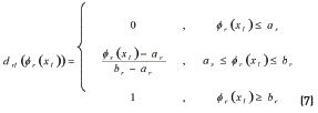
Where b_r corresponds to the most desirable case and a_r to the least desirable case and must be set by the engineer.

Moreover, each element of the penalty function (6) can be expressed as expression (8):

Each response y_r has a target value τ_r and a lower and upper limit given by L_r and H_r respectively, in which . For chromosome x_l to be feasible, the corresponding response must be within those limits (). The constant c avoids p_r from becoming zero if infeasible cases arise, and thus, ensures that a non-zero P is calculated for a non-feasible solution (see [13]). A value of 0.0001 is assigned to c, which does not influence the value of the final solution [13]. To use similar expressions to Eq. (4) to establish the MOP and necessary dominance relations between pairs of chromosomes (solutions) for multiresponse systems, the PGA defines for those systems (see Eq. (9)):

where in (9) D₁ is the desirability (see eq. (5)) corresponding to mean adjustment and D₂ to variance reduction, aggregated across the R responses.

Thus, using (9) and noting that the PGA must maximize f₁(x_l) and f₂(x_l), the MOP for multiresponse systems and corresponding dominance relations between two solutions are as shown in Eq. (10):

and x₁ will dominate x₂ if and only if the conditions in (11) are satisfied:

2.2. Evaluation of the relative efficiency using DEA

DEA is used to calculate the relative efficiencies of the responses obtained by the PGA. DEA is a nonparametric method of operations research for estimating production frontiers of a set of Decision Making Units (DMU). Based on the work of [11, 15] used DEA to measure the relative technical efficiency of DMUs, with multiple inputs and outputs. The measurement of technical efficiency oriented to inputs identifies the quantity to which the inputs must be reduced, for keeping the specified level of the outputs. Correspondingly, DEA can also find the increase in the level of outputs, using the same level of inputs.

As we are interested in assessing the merit of each of the solutions obtained given a choice in the mean deviation and standard deviation and that it cannot be expected a proportional effect in the output due to a change in the inputs, the input-oriented model with variable returns to scale is more appropriate than the output-oriented model. The input-oriented model with variable returns to scale can be defined as follows: Given D DMUs, producing Q outputs, using I inputs, Eq. (12) presents the Charnes, Cooper and Rhodes' model [11, 15, 16] oriented to inputs and variable return to scale, for the case of the DMU d:

where the scalar 0≤E≤1 is the technical efficiency measurement of DMU d, d =1,…, D; Z is the matrix of products z_qd, q = 1,…, Q, K is the matrix of inputs k_id , i = 1,…, I, and λ is a column vector variable with all values non-negative. A fully efficient solution should have E = 1.

Using the notation of the PGA problem described in Section 2.1, Z can be the solution expressed in each chromosome that should be achieved by the system. Taking for instance the following example, in which we need to adjust the width of the painted strip of a car painting system to a nominal width of 40.0 [cm]. In that case, considering each solution achieved by the PGA as a DMU, the vector Z will be replaced by the vector of solutions achieved by the PGA. Correspondingly, the K vector of inputs consists of the vector of mean deviation from the target: │Y-τ│(with τ= 40.0 [cm]) and the vector of standard deviation s of the painted strip achieved by each solution found by the PGA. The constraints Zλ_d ≥ z_d and Kλ_d ≤ E_dk_d define the technology frontier for the observed output vectors z_d and the observed input vectors k_d. The summation 1^T λ = 1 together with the non-negative condition of the λ imposes a convexity condition on how the inputs and outputs of the units can be combined [16]. 

The technical efficiency of each solution delivered by the PGA will be computed and the solutions ranked according to their respective technical efficiencies.

The corresponding will be done for multiple response systems, each solution obtained by the PGA delivers a set of outputs f₁(x_l) and f₂(x_l). The responses f₁(x_l) and f₂(x_l) can be used to build the matrix of outputs Z while the inputs still form the matrix K respectively. Again, the technical efficiency of each solution delivered by the PGA can be computed and the solutions ranked according to their respective technical efficiencies.

2.3 Optimal combination of inputs

The last step of our framework is the selection of the combination of inputs that can be improved in order to achieve a predefined quality measure. In particular, we use the model developed by [17], described by Eq. (13):

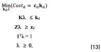
where c_d is the cost vector of DMU d.

For the robust design application, we can first define c_m as the economic cost incurred per unit of mean adjustment (i.e., c_m = $ monetary unit / unit in which mean adjustment is measured) and c_s as the economic cost incurred per unit of standard deviation (i.e., c_s = $ monetary unit / unit in which the standard deviation is measured). These costs may be established by the firm's Quality Assurance Department. For simplicity, the relative cost of mean adjustment to standard deviation can be considered and select the solutions with that minimum relative cost. Thus, using model (13) the vector c_d can be constructed by assigning the relative cost c to the mean adjustment, and cost 1.0 to the standard deviation, while the matrix of responses Z and the matrix of inputs K are the same as defined in Section 2.2. Thus, the model (13) can be used to select the solution with minimum relative cost (i.e. the one which allows incurring the minimum penalty, in economic terms) for each decision unit, in this case, for each solution achieved by the PGA. Once the values are obtained, the solutions can be ranked by their total cost (the objective function of problem (13)) and the less costly solution can be selected.

3. Examples of the application of DEA to analyze the solutions found by the PGA

To apply the proposed DEA method to the evaluation of the solutions delivered by the PGA, two case studies were used. The first one corresponds to a real application of robust design to adjust the automatic body painting process in a car manufacturing plant. The second case study uses a multiresponse process simulator with four responses, ten control factors and five noise factors. This simulator is described in [18].

3.1. Analysis of the solutions obtained for the single-response real system

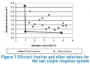
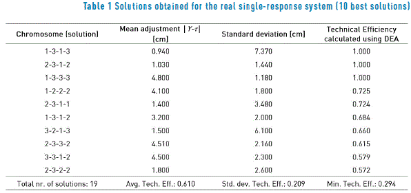
In this case, a robust design experiment was carried out to adjust the width of the painted strip of a car painting system to a nominal width of 40.0 [cm]. The design of the experiment consisted of an orthogonal array L₉(3⁴) for the four control factors and a L₄(2³) for the three noise factors. More details and the data may be found in [19, 20]. Figure 1 shows a graph of the solutions delivered by the PGA. The solutions are plotted using │Y-t│as a measure of mean adjustment and s (the standard deviation) as a measure of variation. Note that we use │Y-t│ instead of (Y-t)² to only have a smaller measure of mean adjustment, and thus make more readable graphs. However, the PGA always uses (Y-t)² in its fitness function. The figure shows the solutions that lie on the efficient frontier along with other solutions found. Table 1 presents the relative technical efficiency of the 10 highest efficiency solutions. In Table 1, the solutions correspond to the combination of the control factors. For example, solution [2-3-1-2] means that the combination of control factors A = 2 (spray gun type 2), B = 3 (paint flow of 390 [cc / min]), C = 1 (fan air flow of 260 [Nl / min]) and D = 2 (atomizing air flow of 330 [Nl / min]) should achieve a painted strip with a mean width of 41.03 [cm] (mean adjustment is 1.030 [cm], and thus y_avg = 40 [cm] + 1.030 [cm]) and a standard deviation of 1.440 [cm]. As expected, the three solutions that lie on the efficient frontier have technical efficiency equal to 1.0. Thus, we can corroborate that the approximation to the Pareto frontier delivered by the PGA is good.

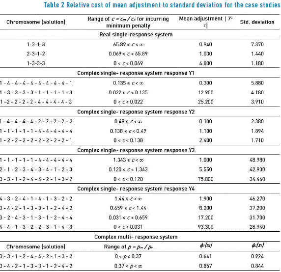
The rest of the solutions shown in Table 1 have efficiencies below 0.73, and thus are not Pareto efficient. Without regard to other considerations, the engineers should select among the three different efficient solutions, the one to be implemented in the system. However, depending on the cost to implement each solution, that decision may be different. In that regard, using model (13) and knowing the economic cost or penalty per unit of mean adjustment (c_m) and the economic cost or penalty per unit of standard deviation (c_s), DEA can determine the efficient solution with the smallest combined cost or penalty. The c_m and c_s economic costs or penalties may be furnished by management, based on the contract signed with the client, i.e. the importance to customers to get products and/or services with a maximum mean adjustment and variation; the cost of implementing each solution in the system; the cost to the firm when achieving a certain level of mean adjustment and variation in its products and/or services, and/or any other consideration. For example, for any of the above-mentioned reasons, management may calculate that for each [cm] that the painted strip is out of the target value of 40 [cm], the firm will incur in a cost of 300 [US$/cm] (c_m), due to the overspraying of the surfaces and thus, the additional paint used. On the other hand, for each [cm] of standard deviation of the painted strip, the cost may be 2,000 [US$/cm] (c_s), because if a high variation exists, that may cause serious quality problems and much rework to be done. For those values, the relative cost is c = c_m / c_s = 0.15. Then, the engineer will set up model (13) using that value of c, and the model will select the solution with the minimum cost. Actually, model (13) will deliver the corresponding mean adjustment and standard deviation attained by that solution. On the other hand, using model (13) the ranges of relative costs c can be computed, within which each of the efficient solutions provides the best alternative (i.e. the minimum penalty value in economic terms). Table 2 shows those ranges. For this system and the above-mentioned considerations, Table 2 indicates that the engineers should select solution [2-3-1-2]. Incidentally, [19] states that the engineers indeed valued more achieving a painted strip with low variation rather than one with a very good mean adjustment. Additionally, given that solution [2-3-1-3] was less expensive to implement than solution [2-3-1-2], they chose the former one [19]. Although [19] does not give economic data in his paper, using model (13) the cost c for that solution can be computed, which is 0.158. That cost means that indeed the engineers valued much more attaining a low variation than a good mean adjustment, determination that is aligned to the recommendation of several practitioners of quality improvement [21]. Remarkably, using model (12), the technical efficiency calculated for that solution is 1.0, achieving a mean adjustment of 6.067 [cm] and a standard deviation of 0.6442 [cm] of the painted strip. From Table 1 and Figure 1, it can be seen that the PGA did not find that extreme solution. This is not surprising, because PGAs find only approximations to the efficient frontier and tend to miss extreme solutions [22].

Notwithstanding all the aforementioned considerations, if for any reason, the manager decides to select a solution that does not belong to the efficient frontier (i.e. an inefficient solution), he /she can consult the technical efficiency of it to assess the decrease in efficiency brought about by his/her decision. For example, if the manager chooses solution [2-3-1-1], then the technical efficiency will be 0.724 (see Table 1), a 27.6% less than if he/she had selected any of the efficient solutions. Additionally, the increment in penalty incurred by implementing solution [2-3-1-1] instead of the efficient solution [2-3-1-2] is high. Using c_m = 300 [US$/cm] and c_s = 2,000 [US$/cm] (the same applied in the previous analysis), the penalty for solution [2-3-1-1] is equal to: c = 300 [US$/cm] x 1.4 [cm] + 2,000 [US$/cm] x 3.48 [cm] = US$ 7,380, where the mean adjustment and standard deviation was obtained from Table 1. On the other hand, the penalty for solution [2-3-1-2] is: c = 300 [US$/cm] x 1.03 [cm] + 2,000 [US$/cm] x 1.44 [cm] = US$ 3,189. The difference between both penalties is US$ 4,191 or the penalty for solution [2-3-1-1] is 2.134 times higher than that for solution [2-3-1-2].

3.2. Analysis of the solutions obtained for the single-response complex systems

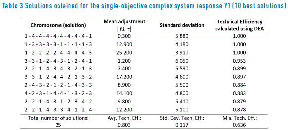
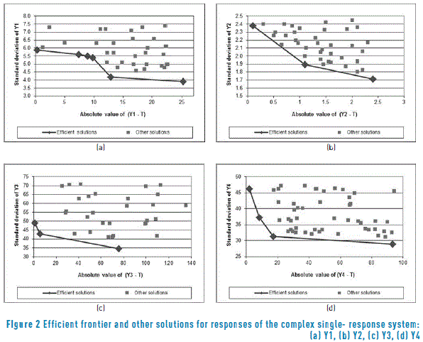
To apply the DEA analysis to a more complex situation, a simulator was used, which is described in detail in [18]. The robust design for this situation considers using an inner array L₆₄(4¹⁰) for the ten control factors and an outer array L₁₆(4⁵) for the five noise factors. For the following case studies, the four responses of the simulator are optimized independent from each other, so that the DEA analysis is applied to the results delivered by the PGA for four single-response systems. Table 3 presents the efficiencies of the best 10 solutions found by the PGA for response one of the system simulator and Figure 2(a) shows a graph of those solutions. Note that three solutions that were regarded as efficient by the PGA, do not have a DEA efficiency equal to 1.0, although their efficiency is very good. This can be clearly seen in Figure 2(a), where the approximation to the efficient frontier found by the PGA is not totally convex. Here again, this result is not surprising because the PGA finds an approximate Pareto frontier and given that it is working with few input data points, its estimation could be modest [22]. The worst solution (not shown in Table 3) has an efficiency of 0.636 and the average efficiency for all 35 solutions found by the PGA is rather good (0.803). On the other hand, as stated before, using model (13) the ranges of relative costs c can be computed, within which each of the efficient solutions provides the best alternative (i.e. the minimum penalty value in economic terms). Table 2 shows those ranges. Those ranges indicate the solution that should be selected by management, according to the relative importance of mean adjustment and standard deviation for the response, per a similar consideration as the one already presented in subsection 3.1 for the real system.

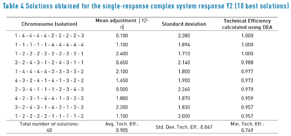
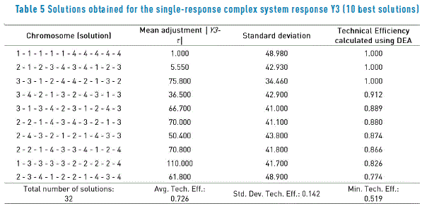
Table 4 and Figure 2(b) show the results for the solutions found by the PGA for response two of the single-objective complex system. Here the DEA analysis indicates that the PGA found a good approximation to the efficient frontier and that the 40 solutions delivered are good, as suggested by an average efficiency of 0.905 and a minimum one of 0.749. The same can be said regarding the solutions for response three, whose values are shown in Table 5 and depicted on Figure 2(c).

The solutions for response three are somewhat inferior to those for response two, since the average efficiency for the 32 solutions of response three is only 0.726 with a minimum of 0.519. As before, Table 2 presents the ranges of c that help to select among the efficient solutions, the one to be implemented in the system for response two and three.

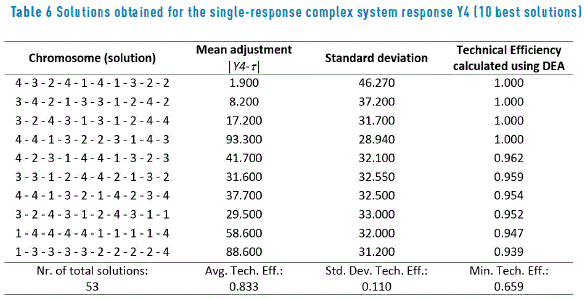
Finally, Table 6 presents the efficiencies for the solutions found by the PGA for response four and Figure 2(d) shows the corresponding graph. For response four, the DEA efficient frontier is defined by four solutions. The average efficiency of the 53 solutions is 0.833 with a minimum of 0.659. Thus, the PGA did well in finding a large number of good solutions. Table 2 shows the corresponding ranges of cost c for helping to select the solution that may best meet the management needs.

3.3. Analysis of the solutions obtained for the multiresponse complex system

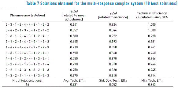
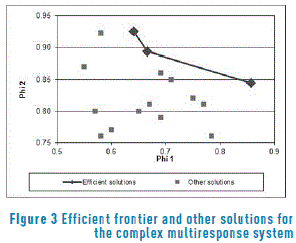
This case study used the same simulator and the same experimental design as before, but the solutions found by the PGA should optimize the four responses at the same time. This means that the PGA is optimizing a four–dimensional multiresponse system. Before presenting the solutions, the reader should bear in mind that for this case, the PGA is maximizing the measures f₁(x_l) (related to mean adjustment) and f₂(x_l) (related to reduction of variation), thus the higher f₁(x_l) and f₂(x_l), the better. The model (13) can be restated to account for this change of purpose by simply replacing the c costs by prices p and maximizing the function. The resulting model is now a maximization problem that calculates the increase in value (expressed in a bonus or price) that a customer gets for incrementing f₁(x_l) and f₂(x_l) (i.e. getting a tighter mean adjustment and a smaller variation). The prices p will be used by the management of the system in the same way that the c costs were used, but from a strict conceptual economic point of view, the aforementioned difference is worth noting. Table 7 and Figure 3 present the results and corresponding graph of the solutions found by the PGA. Since this is a maximization problem, the frontier should be concave and the non-efficient solutions should lie to the left of that frontier. Note that the frontier is not totally concave and that the middle solution of the frontier should not belong to it. That solution [2 - 1 - 2 - 3 - 4 - 3 - 4 - 1 - 2 - 3] withf₁(x_l) equal to 0.665 and f₂(x_l) equal to 0.893, has a DEA efficiency of 0.981. Thus, it is near the frontier, but strictly speaking is not part of it. Here again, the PGA found a reasonable approximation to that frontier, but due to the small number of input data points, the approximation may be modest [22].

Using model (13) for this case, the ranges of relative prices p can be computed, within which each of the efficient solutions provides the best alternative (i.e. the maximum economic benefit). Table 2 shows those ranges. For example, if management estimates that the price p_m clients may pay for mean adjustment relative to the price for reduction in variance p_v is p = p_m / p_v = 0.3, then they should select solution [3 - 3 - 1 - 2 - 4 - 4 - 2 - 1 - 3 - 2]. In that case, management believes that clients value more variance reduction than mean adjustment. On the contrary, if the estimate of p is for example 1.5, that means that customers value more mean adjustment than variance reduction and solution [3 - 4 - 2 - 1 - 3 - 3 - 1 - 2 - 4 - 2] should be selected.

4. Conclusions

The analyses of the solutions found by the PGA for all the case studies using DEA's model (12) show that the approximation to the efficient frontier found by the PGA is rather good. Additionally, and perhaps more important, DEA's model (13) will help decision makers to make the right decision regarding the solution to be selected for being implemented in the system. In the case of single-response systems, by estimating c_m (the cost or penalty of achieving a certain value of mean adjustment) and c_s (the cost or penalty of getting a given standard deviation), the approach presented can clearly show the trade-off between mean adjustment and variation reduction in the production and/or service process and thus management can consciously select the alternative that better meets a specified quality level. For multiresponse systems, the same can be said, but using the prices p_m and p_v. In any case, if for any reason, a solution that does not lie on the efficient frontier is selected, the presented approach can be used to compare the technical efficiencies and penalties of the solutions, so that management can clearly assess the relative downgrading of those values.

Finally, because the DEA analyses of the solutions delivered by the PGA show that the algorithm seems to work reasonably well in the case studies, it is meaningful to continue developing and improving it. One of such enhancements could be to try to achieve a better approximation of the efficient frontier, both in terms of obtaining more points of the frontier and a more convex or concave one. Although robust design studies use highly fractioned experimental designs to reduce experimental costs, and thus the PGA works with a relatively small number of data points, the PGA could try to counterbalance that by using additional points calculated by response surface methodology (RSM) [23]. In this case, RSM may be applied for estimating the response surface of the system using the experimental data and then employing the response surface to calculate additional points that will be used by the PGA. The authors are working on such improvement and preliminary results show that such refinement is worth investigating.

5. Acknowledgements

This work was funded in part by Fondecyt (Fondo Nacional de Ciencias y Tecnología of the Chilean Government) grant N° 1130052 to the first author.

6. References

1. G. Taguchi, Systems of experimental design, 4^th ed. Dearborn, USA: American Supplier Institute, 1991.         [ Links ]

2. T. Robinson, C Borror and R. Myers, ''Robust Parameter Design: A Review'', Quality & Reliability Engineering Internation, vol. 20, no. 1, pp. 81-101, 2004.         [ Links ]

3. H. Allende, E. Canessa and J. Galbiati, Diseño de experimentos industriales, 1^st ed. Valparaíso, Chile: Universidad Técnica Federico Santa María, 2005.         [ Links ]

4. H. Allende, D. Bravo and E. Canessa, ''Robust design in multivariate systems using genetic algorithms'', Quality & Quantity, vol. 44, no. 2, pp. 315-332, 2010.         [ Links ]

5. S. Maghsoodloo and C. Chang, ''Quadratic loss functions and signal-to-noise ratios for a bivariate response'', Journal of Manufacturing Systems, vol. 20, no. 1, pp. 1-12, 2001.         [ Links ]

6. W. Wan and J. Birch, ''Using a modified genetic algorithm to find feasible regions of a desirability function'', Quality & Reliability Engineering International, vol. 27, no. 8, pp. 1173-1182, 2011.         [ Links ]

7. J. Holland, Adaptation in Natural and Artificial Systems: An Introductory Analysis with Applications to Biology, Control, and Artificial Intelligence, 1^st ed. Ann Arbor, USA: MIT Press, 1974.         [ Links ]

8. C. Lin, C. Anderson, M. Hamada, L. Moore and R. Sitter, ''Using Genetic Algorithms to Design Experiments: A Review'', Quality & Reliability Engineering International, vol. 31, no. 2, pp. 155-167, 2015.         [ Links ]

9. B. Forouraghi, ''A Genetic Algorithm for Multiobjective Robust Design'', Applied Intelligence, vol. 12, no. 3, pp. 151-161, 2000.         [ Links ]

10. E. Canessa, G. Bielenberg and H. Allende, ''Robust Design in Multiobjective Systems using Taguchi's Parameter Design Approach and a Pareto Genetic Algorithm'', Rev. Fac. Ingeniería Univ. Antioquia, no. 72, pp. 73-86, 2014.         [ Links ]

11. A. Charnes, W. Cooper and E. Rhodes, ''Measuring the Efficiency of Decision Making Units'', European Journal of Operational Research, vol. 2, no. 6, pp. 429-444, 1978.         [ Links ]

12. D. Aigner, C. Lovell and P. Schmidt, ''Formulation and Estimation of Stochastic Frontier Production Function Models'', Journal of Econometrics, vol. 6, no. 1, pp. 21-37, 1977.         [ Links ]

13. F. Ortiz, J. Simpson, J. Pigniatello and A. Heredia, ''A Genetic Algorithm Approach to Multiple - Response Optimization'', Journal of Quality Technology, vol. 36, no. 4, pp. 432-450, 2004.         [ Links ]

14. E. Castillo, D. Montgomery and D. McCarville, ''Modified Desirability Functions for Multiple Response Optimization'', Journal of Quality Technology, vol. 28, no. 3, pp. 337- 345, 1996.         [ Links ]

15. M. Farrell, ''The Measurement of Productive Efficiency'', Journal of the Royal Statistical Society Series A General, vol. 120, no. 3, pp. 253-290, 1957.         [ Links ]

16. W. Cooper, L. Seiford and K. Tone, Data Envelopment Analysis: A Comprehensive Text with Models, Applications, References and DEA-Solver Software, 2^nd ed. New York, USA: Springer, 2007.         [ Links ]

17. R. Färe, S. Groskopf, C. Lovell, The Measurement of Efficiency of Production, 1^st ed. Boston, USA: Kluwer-Nijhoff Publishing Co., 1985.         [ Links ]

18. E. Canessa, C. Droop and H. Allende, ''An improved genetic algorithm for robust design in multivariate systems'', Quality & Quantity, vol. 46, no. 2, pp. 665-678, 2011.         [ Links ]

19. W. Vandenbrande, ''Make love, not war: Combining DOE and Taguchi'', in ASQ's 54^th Annual Quality Congress Proceedings, Indianapolis, USA, 2000, pp. 450-456.         [ Links ]

20. W. Vandenbrande, ''SPC in paint application: Mission Impossible?'', in ASQ's 52^nd Annual Quality Congress Proceedings, Indianapolis, USA, 1998, pp. 708-715.         [ Links ]

21. K. Ranjit, Design of Experiments Using the Taguchi Approach: 16 Steps to Product and Process Improvement, 1^st ed. New York, USA: J. Wiley & Sons, 2001.         [ Links ]

22. K. Deb, L. Thiele and E. Zitzler, ''Comparison of Multiobjetive Evolutionary Algorithms: Empirical Results'', Evolutionary Computation, vol. 8, no. 2, pp. 173-195, 2000.         [ Links ]

23. R. Myers, D. Montgomery and Christine M. Anderson, Response surface methodology: process and product optimization using designed experiments, 2^nd ed. New York, USA: J. Wiley & Sons, 2002.         [ Links ]