


 English (pdf)
 Article in xml format
 Article references
 Send this article by e-mail
 Cited by SciELO
  Cited by Google
  Similars in
SciELO
Similars in
SciELO  Similars in Google
 Permalink
1. Introduction
There are numerous applications in different study areas where the generation of homogeneous and controlled magnetic fields are required, one of these is the research in bioelectromagnetics[1-3]. Many of these studies ideally require devices capable of generating uniform magnetic fields and furthermore guaranteeing a controlled and repeatable exposure to different samples involved in the experiment[4,5]. In this sense, the arrangements of air-core coils have been traditionally used for this purpose, particularly circular and square geometries[6-8].
On the other hand, the magnetic field control systems attempt to compensate the ambient magnetic field components capable of generating changes on the desired magnetic field distribution on a specific volume, this compensation can be achieved through an active or passive (shielding) system[9]. Active compensation consists in generating a magnetic field in opposite direction to the reference magnetic field in order to compensate the ambient magnetic field components[10], including the geomagnetic field[11], resulting in the desired magnetic field without interference.
The main advantage of the active compensation system is that not only can it be used in shielding applications but it also allows adjustment of magnetic field levels different to zero; this involves in most cases that the system also incorporates, in addition to the generation system, the use of sensors and a control system to achieve a controlled magnetic field distribution on the volume of interest[12,13]. Magnetic field compensation systems are used in different applications such as microscopy, diagnostic imaging, positioning, magnetic fields measurement, electromagnetic stimulation, etc.[14-18].
Systems such as MEDA[14], Park et al.[16] and Raganella et al.[17] use, in most cases, a computer system as a magnetic field control unit. On the other hand, Novickij et al.[18], Malafronte and Martins[19] and Farina et al.[20] use a microcontroller system to generate a controlled magnetic field in a specific direction and magnitude, but these do not specify what kind of control laws were used. In this paper a simple geomagnetic field compensation system based on a microcontroller for uniform magnetic field applications of low magnitude and frequency is proposed; it starts with the coils system description, continuing with the validation using a simulation software based on Finite Element Method (FEM) and ending with experimental results of the geomagnetic field compensation on the volume of interest. The proposed system emerges as a low-cost and portability alternative for the generation of controlled magnetic fields unlike other works[17-20] not only single axis with geomagnetic compensation but also the generation of controlled magnetic fields up to 200 µT on all magnetic field components Bx,y,z around a specific volume without the need of additional sensors for magnetic field compensation such as the MEDA system[14].
2. Methodology and systems
The methodology is based on the design, implementation and validation of the geomagnetic field compensation system. Firstly, the design is divided into three components: generation, measurement and control of magnetic fields; the generation is based on the mathematical analysis of the generated magnetic field by a finite wire in a square loop using the Biot-Savart law; the measurement consists in selecting and specifying the sensor to use, taking into account the constraint of low magnitude and frequency (geomagnetic field); and lastly the control is based on the selection of the microcontroller device and the control law specification. The generation and measurement components were validated by simulation and using a Gaussmeter respectively. Finally, the implementation, integration and validation of the geomagnetic field compensation system are performed, considering the physical and electric parameters for the experimental tests of the magnetic field control and the geomagnetic field compensation.
The proposed system is controlled using an active compensation technique and is mainly composed of three parts: the generation system of uniform magnetic fields which consists of an array of Tri-axial Square Helmholtz (TSH) coils; the measurement system built with AD22151 Hall effect magnetic field sensors in a tri-axial configuration and the control and coupling system based on the ATMega16 microcontroller, as shown in Figure 1. The system operation principle is based on the magnetic field compensation on each coordinate axis (x, y, z) in order to obtain a global compensation on the volume of interest[17]. Therefore, the measurement of each magnetic field component B x , B y and B z is necessary to counteract the ambient magnetic fields effects (natural and/or artificial)[21].
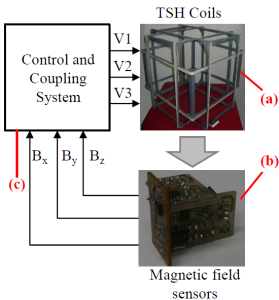
Figure 1 Geomagnetic field compensation system: (a) Generation system of uniform magnetic fields. (b) Measurement system. (c) Control and coupling system
2.1. TSH coils system
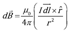
The TSH coils system[6] consists of an array of three square Helmholtz coils pairs as shown in Figure 1(a), where each pair is located on each coordinate axis (x, y, z). The study of the behavior of the magnetic field B generated by the square Helmholtz coils is made using the Biot-Savart law [22,23] for each finite wire as presented in Eq. (1), where dl is an infinitesimal segment of the current loop, I is the current through the loop, μ
0
is the permeability of the free space, r is the distance from an extreme of the current loop to the evaluated point and is a unit vector.
 (1)
(1)
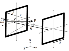
Helmholtz configuration consists in a pair of coils located parallel on either side of the test area along a common axis (in this case z-axis), spaced at a distance h as shown in Figure 2 [23]; where each black thick line represents a square coil of conductive wire, a is the half side length of the coil, P is the evaluated point and s is the perpendicular distance from the current loop axis ( on x-axis) to P. Each coil consists of N turns and the relationship between the side and the separation distance for square Helmholtz coils is given by a factor of 0.5445 (h=1.089a)[6], these physical parameters depend on the restrictions of the application in terms of the desired volume with a uniform magnetic field. The square coils are connected in series generating a highly uniform magnetic field on the axis of symmetry (z-axis); therefore solving (1) for x=y=0 the resultant magnetic field is equal to the B
z
component because the other (B
x
and B
y
) components are zero [23] and it is calculated by the following Eq. (2):
on x-axis) to P. Each coil consists of N turns and the relationship between the side and the separation distance for square Helmholtz coils is given by a factor of 0.5445 (h=1.089a)[6], these physical parameters depend on the restrictions of the application in terms of the desired volume with a uniform magnetic field. The square coils are connected in series generating a highly uniform magnetic field on the axis of symmetry (z-axis); therefore solving (1) for x=y=0 the resultant magnetic field is equal to the B
z
component because the other (B
x
and B
y
) components are zero [23] and it is calculated by the following Eq. (2):
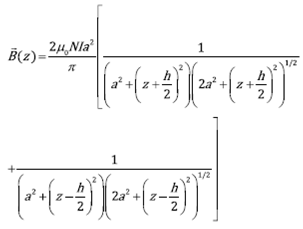 (2)
(2)
In this research, the design of the TSH coils was dimensioned for studies on biological systems in vivo and in vitro; that is, allowing the experimentation with cellular culture plates, small animal or small seeds[6]. The side lengths defined were 0.56 m, 0.58 m and 0.60 m on each symmetry axis x, y and z respectively.
2.2. Magnetic field measurement system
The magnetic field sensors are placed orthogonally to each other in order to obtain the measurement of the magnetic field intensity in the three coordinate axes B x , B y and B z , allowing the magnitude of the resulting magnetic field (B r ) to be determined[24] as presented in the following Eq. (3):
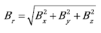 (3)
(3)
The experimental array for the detection of each magnetic field component was designed in a modular way to allow a practical assembly and the necessary perpendicularity to obtain the measurement of the resulting magnetic field. The most important advantage of the measurement system illustrated in Figure 1(b), in addition to its low cost[25], is the implementation with surface mount devices and the possibility of having two measurement ranges +10 mT and +2 mT through a selector, these characteristics allow the size of the experimental assembly to be minimized.
Moreover, the sensors should be placed in an appropriate location and orientation on the region or point to be measured in order to guarantee a reliable measurement of the magnetic fields. Nevertheless, it is recommended to keep the sensors configuration without any obstacle around the encapsulation surface, in order to avoid disturbances in the process of measuring.
2.3. Control and coupling system
Figure 3 shows the control and coupling system which is divided into several components such as the amplification and conditioning stage, microcontroller, Digital/Analog Converters (DAC) and power stage.
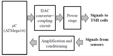
The amplification and conditioning stage allows the voltage signals delivered by the sensors to be adjusted, of the measured magnetic fields, within limited values to be digitized by the Analog/Digital Converters (ADC) of the microcontroller. Meanwhile, the ATMega 16 microcontroller is in charge of the digital processing of the measured variables and the calculation of the control actions.
The controlled variables are converted into analog signals using the DAC7625P 12 bits converter and finally, these voltage signals are delivered to the TSH coils via the power stage based on the OPA549 operational amplifier of the Texas Instruments company which has characteristics of high electric current operation, protections of temperature and adjustable overcurrent [26]
The measured variables become the feedback signals of the control system and depending on the reference or desired values, the respective controls on the electric variables that modify the generated magnetic fields by the TSH coils are applied. In this case, the controlled variables are the voltages applied to each pair of square Helmholtz coils (V1, V2 and V3); it must be bipolar in order to generate magnetic fields in both directions.
The difference between the reference and measured magnetic fields is called error e(k). The control actions implemented with the microcontroller u(k) are based on permanent calculation of the errors to determine the voltage values to be applied to the TSH coils system, these values are calculated and updated by the difference Eq. (4) for a proportional gain (K p ), an integration time T i and a sampling period T s [26]. This expression is a proportional and integral control action (PI), which is the most commonly used technique in feedback systems to remove the steady state error[27].
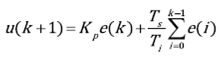 (4)
(4)
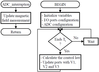
A continuous comparison between the reference and measured signals is performed by the digital control system. If the reference signals are greater than the measured, the control system will increase the generated magnetic fields by the TSH coils. Likewise, if the reference signals are less than the measured, the control system will reduce the generated magnetic fields by the TSH coils. Eventually, in steady state conditions the difference between both magnetic fields will be insignificant, ideally zero. The flowchart of the program in the microcontroller is shown in Figure 4, where the ADC interruption routine that update the measurements and the main routine can be observed.
3. Results and discussion
The proposed compensation system aims to compensate for small variations of the ambient magnetic field (natural and/or artificial) that may generate a change in the magnitude of the desired magnetic field on the volume of interest. In this section, the validation by simulation of the generation system and the experimental results of the magnetic field control and the geomagnetic field compensation are presented.
A FW Bell Gaussmeter (5170) for validation of the measurement system owned of the High Voltage Laboratory at Universidad del Valle, which has calibrations required according to the standards was used. For the system experimental tests a voltage source (GPC-3030D), a digital multimeter (ET-2110) and an oscilloscope (DS1202CA) were used. The power system responsible for energizing the TSH coils can supply + 25 V at 3.5 A. Finally, the experimental results were obtained for operating conditions without biological material.
3.1. Uniform magnetic field
In order to verify the distribution and uniformity of each magnetic field component B x , B y and B z on the volume of interest, a 3D computational model in COMSOL Multiphysics® was designed (see Figure 5]. The TSH coils computational model consists of three pairs of square Helmholtz coils and a sufficiently large cube to which the zero potential for electromagnetic analysis using the AC/DC module is assigned[28].
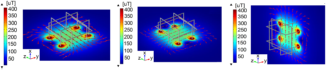
Figure 5 Simulation of magnetic field flux lines and uniform area in the TSH coils: (a) Pair 1-B z . (b) Pair 2-B y . (c) Pair 3-B x
Taking into account the design parameters (physical and electrical) and operational conditions of the TSH coils system (N=50 turns, electric current for each pair of coils 1.5 A, 1.45 A and 1.4 A from the largest to the smallest respectively), the simulation is performed energizing each pair of coils independently (to obtain B x,y,z =200 µT), generating the contour maps of the magnetic flux density shown in Figure 5. Furthermore, the direction of the magnetic field lines and the uniformity region over the center of separation of the coils are shown[6].
Experimental results[6] ensure an average cubic volume of side length 0.12 m (homogeneity 0.45 %) with uniform magnetic field around the center of the TSH coils. The average measured magnetic field obtained was 204 μT in the center of separation of each coil pair. The maximum error found between measured and simulated values was 7.4 %, this error is associated in part to the uncertainty of the measurement process (ambient conditions, resolution of measuring equipment, etc.) and the numerical methods (mathematical approaches) used by the simulation software to find the solution. Finally, the resolution of the measurement system was 1 μT.
3.2. Magnetic field control
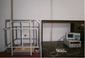
The complete system configuration is shown in the experimental arrangement of Figure 6 where the control and coupling system can be observed, TSH coils system, measurement system and auxiliary equipment of power and registration. The system operation can be in open or closed loop depending on the application. The open loop operation is limited to the generation of a uniform magnetic field on each coordinate axis without control. Meanwhile, the closed loop operation allows the control of the generated magnetic field on each coordinate axis, giving the possibility of attenuation of the ambient magnetic fields such as the geomagnetic field.
The operation of the magnetic field control system by setting a reference value of 0.1 mT in the B z component was checked. Therefore, the control action is made on the applied voltage to the pair 1 of the TSH coils system (see Figure 5(a)). Figure 7 shows the response of the magnetic field control system to a reference value of 0.1 mT, where a good monitoring of the reference signal can be observed with a steady state error close to zero and a stabilization time approximately 0.24 seconds. This stabilization time is due to the restriction of the maximum change of the output voltage which was set at +1 V, in order to avoid high voltage peaks and large variations in the electric current of the coils.
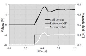
Moreover, the control system is capable to counteract a disturbance in the generated magnetic field by the coils; in this case, the disturbance is made by approaching a metallic material (with different permeability of the free space) on the sensor package in order to alter the experimented magnetic field. In general, the results showed a maximum error of 3.2 % between the desired magnetic field and the controlled magnetic field (measured).
3.3. Magnetic field compensation
One of the main features of the magnetic field control system is the possibility to compensate the geomagnetic field or the ambient magnetic fields. In this case, a reference magnetic field equal to 0 mT is adjusted in each magnetic field component B x , B y and B z . Figure 8 shows the results of the geomagnetic field compensation on each coordinate axis (x, y, z).
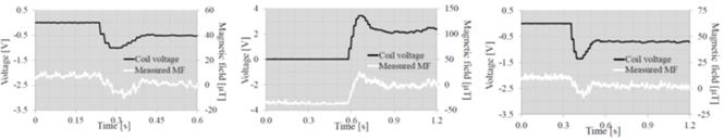
Figure 8 Geomagnetic field compensation on the coordinate axes: (a) Pair 1-B z . (b) Pair 2-B y . (c) Pair 3-B x
Importantly, the horizontal component of the terrestrial magnetic field (B TH ) was located on the zy plane, corresponding to the symmetry axes of the pairs 1 and 2 of the TSH coils system as shown in Figure 5(a) and Figure 5(b) respectively. Therefore, the average value of B TH experimentally obtained was 38.1 µT; this value is constantly changing due to small variations that naturally occur during the day[29]. Furthermore, due to artificial magnetic fields generated by electrical equipment close to the measurement region such as computers, voltage sources, lighting systems, etc.
The results in Figure 8 allow verifying the correct functioning of the geomagnetic field compensation system. The obtained magnitudes of the magnetic field components were B z =6.3 µT, B y =37.6 µT and B x =10.2 µT respectively. These values were compensated and a uniform volume with magnetic field approximately equal to 0 mT was obtained.
Control systems based on microcontroller are used in several applications[25-30] such as power electronics, healthcare equipment, mobile applications, among other; as a low-cost solution due to the portability, low-power consumption and high performance depending on the application. The presented system is a low-cost solution based on a microcontroller that allows the generation of controlled magnetic fields up to 200 µT on all the magnetic field components B x,y,z around a specific volume for uniform magnetic field applications. This system can be compared with Raganella’s system[17] which uses a PC as control unit for generation of controlled magnetic fields considering a similar homogeneity and generation range. On the other hand, low-cost solutions based on microcontroller were studied by Novickij et al.[18], Malafronte and Martins[19] and Farina et al.[20] for the controlled magnetic field generation but only for single axis, while the three-axis compensation system such as MEDA[14] presents high costs and limitations in the ability to counteract changes in the ambient magnetic field.
4. Conclusion
A simple geomagnetic field compensation system based on a microcontroller and the integration of the TSH coils system with orthogonal sensors was built. This low-cost system allows through a simple control not only the generation of a controlled magnetic field but also the compensation of the geomagnetic field or the ambient magnetic fields (several µT) on all the components around a uniform volume. Several electromagnetic stimulation studies of low magnitude and frequency for in vivo or in vitro biological experiments with different approaches can be performed.

