


 Inglês (pdf)
 Artigo em XML
 Referências do artigo
 Enviar este artigo por email
 Citado por SciELO
  Citado por Google
  Similares em
SciELO
Similares em
SciELO  Similares em Google
 Permalink
1. Introduction
Resilience and stability refer to the ability of an ecosystem to withstand and recover from perturbations [1-6]. Resilience is a measure of the ability of systems to absorb changes and still persist [3, 7]. In general terms, resiliency refers to "out of equilibrium events" [8] and reflects the degree to which a system is capable of rebuilding and increasing its ability to adapt from a disturbance [9-11]. Resiliency can also be interpreted as the time required by the variables to gain back their equilibrium following a perturbation [6, 12].
Stability is defined as the ability of an ecosystem to return to an equilibrium state after a temporary disturbance [3]. Stability refers then to: i) the behavioral patterns followed by a system in the absence of disturbances; ii) the degree to which perturbations can be experienced by the system without interruption of these patterns; and iii) the speed at which the system returns to these patterns once they have been disorganized [5].
The concepts of resiliency and stability are fundamental to assess conservation practices of biological diversity and to ensure long-term intergenerational sustainability of the ecosystems [13], which is the purpose of conservation ecology. Although resilience and stability are different conceptually, both depend on variables such as the amount of both intraspecific and interspecific relationships established in an ecosystem [14], biodiversity [15, 16]; amount of biomass [17], coverage area; water flows; temperature; soil conditions [18], and the imbalance caused by humans [8], among others.
Despite the conceptual clarity of these concepts, one of the major drawbacks for the long-term conservation of ecosystem biodiversity is the lack of information on the resilience and stability of each ecosystem. Conceptual proposals have been made on the assessment of the resilience and stability of natural ecosystems [8, 15, 19, 9] or in coastal ecosystems [20]. Similarly, there have been field approximations around the world, mostly in temperate areas [17] [21, 22]. There is also a need for specific research on the characteristics of ecosystems, the degree of human intervention [23, 24], the degree of invasion, degradation [13], and resilience and stability [2, 25].
Disturbances induce a state shift that modifies biotic interactions and feedbacks within communities, such as competitive dynamics and plant-herbivore interactions [2, 4, 26, 27] When the resilience of an ecological system is exceeded by the disturbances, a regime shift occurs [1].
The recovery assessments of ecosystem dynamics after disturbance do not provide definitive evidence for the existence of a threshold or a quantitative measure of resilience [4]. However, there are algorithms to model the environmental recovery on post-fire events [28, 29] and modeling proposals for ecosystem recovery and behavior under climate change [30, 31], but experimental tests of thresholds associated with disturbances are rare, particularly for terrestrial ecosystems [7].
In this paper, we introduce a spatiotemporal ecohydrological model to address the concepts of resiliency and stability of terrestrial ecosystems from a mathematical perspective. The ecohydrological model combines system dynamics and agent-based algorithms to represent fundamental ecological dynamics (i.e., intra and interspecific interactions), linked to hydrologic variables (i.e., temperature, precipitation and soil water moisture conditions). The model allows the analysis of clearance-type disturbances to assess the resiliency and stability of the simulated ecosystem through indices modified from hydrological analysis in water resources. The paper initially describes the model structure, followed by the results of the simulations, a discussion on the implications of the results and some concluding remarks regarding the use of this kind of models in the assessment of ecosystem conditions.
2. Materials and Methods
2.1. Model Structure
The model is constructed on the basis of a tessellation of squared cells (i.e., a 100(100 cell array), in which each cell interacts according to the Moore neighborhood criterion [32, 33], with discrete time steps representing monthly variations. The model is capable of reproducing the coupled interaction of n populations in the same time and space. Although the model allows the interaction of an unlimited number of plant species, since the model runtime increases as more species are introduced, we show the interactions of ten different populations among them and with the surrounding environment. Each cell can potentially host all the populations, given their dynamic interactions.
The model is composed of two parts (Figure 1):
1. A system dynamics algorithm that determines the monthly water balance and soil moisture conditions at each cell, based on climate-plant-soil interactions.
2. An agent based algorithm that accounts for the intra and interspecific interactions among plant populations in each cell and with its neighboring cells, given the water availability and temperature conditions determined with the first algorithm.
The water-balance algorithm determines the monthly soil moisture condition in each cell given the inputs of monthly rainfall and temperature series and soil characteristics such as wilting point (the minimum water content in each soil type) and field capacity (the maximum water content stored per soil type). Initially, part of the rainfall infiltrates in the soil and part leaves the cell as runoff. Plant evapotranspiration is calculated with the Thornthwaite equation [34] that is still used in different studies [35-38], which considers latitudinal changes of potential evaporation with monthly mean temperatures.
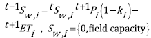
The basic water balance equation in each cell i is therefore defined as (1):
 (1)
(1)
Where the left superindex refers to time intervals t and t+1, S w,i is the soil moisture content on cell i, P i and ET i are the monthly precipitation and evapotranspiration over the cell i and k i is a runoff coefficient defined per cell.
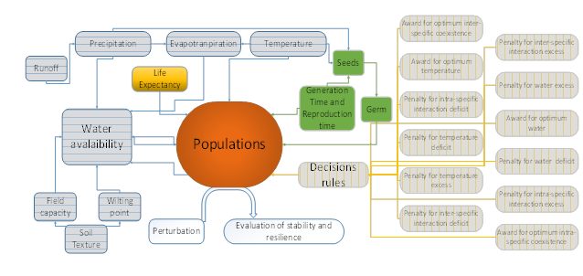
Figure 1 General model structure: water balance in horizontal lines, agent-based decisions in vertical lines. Resilience and stability are evaluated over population scores
The second part of the model corresponds to an agent-based system, which is a versatile modeling tool in ecology [39]. The model uses cellular automata to represent the populations that continuously respond to the simulated abiotic and biotic conditions. Four factors rule the cellular automata (see Figure 1): i) intraspecific relationships (depending on the current states of the same population in adjacent cells), ii) interspecific relationships (depending on the current states of other populations in adjacent cells), iii) temperature (related to ranges of tolerance for each population), and iv) water availability (related to a suitable survival range of each population) (Figure 2).
Each factor receives three possible values (minimum, optimum, maximum), according to the generation time of each population, following power functions. In total, 12 types of values are required to determine whether a population will be present in a cell in the next iteration [Figures 1 and 2]. Other factors, such as generation time, life expectancy, the number of offspring and survival rates, are assigned allometrically, based on the size of the simulated species [40-43]. The model is run monthly for the equivalent of 120 years. Within this period each population is able to reach an equilibrium. The model is programmed in MATLAB ®.
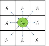
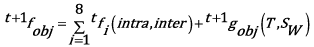
Figure 2 Scheme of agent-based model: objective function f obj is evaluated on each cell, based on its own temperature T and soil water availability S w (function g obj ) and on intra- and inter-specific values from its eight neighboring cells (see factor values in Table 1]
The Figure 2 is represented by the following equation (2).
 (2)
(2)
2.2. Soil texture
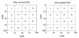
Soil hydraulic properties are defined as a function of soil texture, following [44]. We fit the curves for the original charts of field capacity and wilting point with the software ZunZun [45], to facilitate their incorporation as algorithms in the model. The soil-texture array for simulation in this paper consists of 16 squares of 25(25 cells (Figure 3).
2.3. Potential Evapotranspiration Function (PET)
The model uses the Thornthwaite equation [34, 46], adapted from USGS [47], to calculate the PET. Although more advanced equations are available (i.e., Penman-Monteith), we chose the Thornthwaite equation due to its explicit consideration of latitudinal variations on monthly evapotranspiration rates, which are relevant for the model proposed.
2.4. Rainfall and temperature series
Although the model allows the incorporation of historical series, the analysis is based on synthetic monthly time series of temperature and precipitation stochastically generated using an autoregressive AR(1) process. Initially, these series are considered stationary but the model can incorporate trends to simulate climate change scenarios. Temperature values are uniformly distributed whereas precipitation values are distributed in clusters randomly generated over the grid.
2.5. Perturbation
Perturbations can be modeled as changes in rainfall and temperature patterns, soil texture, cells clearance or changes in species. These perturbations may affect portions of the ecosystem and disturb one or more populations at different times. For the purposes of this paper, we consider cells clearance only as the control perturbation, with 20% and 60% of cells cleared up of populations after having reached the equilibrium stage. We chose these percentages to give a contrasting idea of the effects derived from the size of clearance in the recovery of equilibrium conditions.
2.6. Population Description
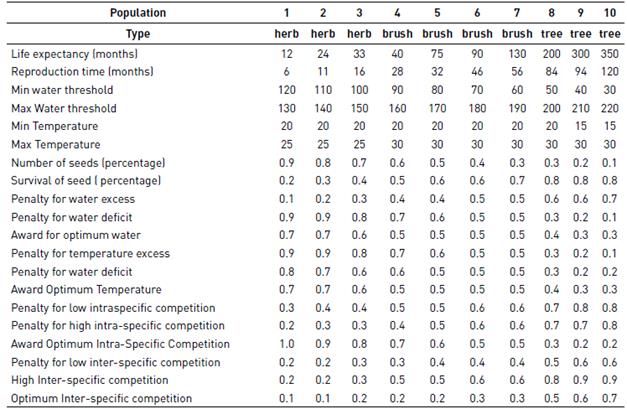
We define populations by allometric relationships in which the weight and size of a species correlates with its reproductive behavior. The allometric relationships between reproductive and vegetative size are common in plants [48]. We established the allometries for each of the plant species in the model, taking into account generation time [40, 42, 49, 50], life expectancy [40], reproduction time [41], and seed quantity [51]. We considered ten plant populations that represent a wide range of possible populations in an ecosystem (Table 1). As a matter of guidance, the ranges for herbs (grasses) tend to show short life expectancies and large reproduction rates, whereas brushes show intermediate values and trees long life expectancies and lower reproductions rates.
We use the generation time law to calculate the time necessary for an individual to grow and mature to reach reproductive age. This law relates the generation time with the body weight of a mature individual at its time of reproduction, in which the species with larger body size usually have longer generation times. The law of generation time was expressed originally by [42, 49] for animal species and modified later by [43] for plant species. Following the later, the law is expressed in the model as:
 (3)
(3)
where g is the average generation time of the population (in years), a is a constant and W is the average body weight of the species (in kgf).
The reproduction time is modeled through the Calder law [41], which describes how species with larger body size usually have longer population cycles. Although originally proposed for mammals, this law is assumed here as valid also for plants. Calder law states that the population cycle increases with increasing size of the body at a power of about 1/4 of the body mass [41].
 (4)
(4)
Where t is the average time of the population cycle, a is a constant and W is the average body weight of the organism.
The life expectancy is defined as the average age in which a species would naturally die off, given other considerations (like water availability and competence) are not stressors. In the model, we calculate life expectancy as a linear relationship of the generation time, which has been described by some researchers as a reasonable assumption [40]. After reaching the expected life, a probability factor is included to calculate the survival of the population in a cell.
2.7. Seed production
Seed production is a factor that largely controls the behavior of each of the populations in the model. We incorporate two types of seed production strategies, known as r and k. The type r plant strategy allocates more efforts to reproduction instead of biomass, which allows a rapid establishment (colonizing ability) on free sites [52]. This strategy produces many seeds with low survival probabilities, with patterns in which the smaller species are "reproductively economic" compared to larger species [53]. The type k strategy invests more energy in few descendants, but with higher survival rates [54, 55]. This strategy produces high biomass and has a greater ability to harvest light and reach other resources and thus has a strong competitive ability [52]. The r and k reproductive types constitute the extremes in the spectrum of adaptation strategies, with most plants and animals manifesting intermediate strategies [52].
The survival of seeds that effectively germinate and become part of the population is modeled through a fertility ratio that depends on the biomass of the parental species. In this way, species with more biomass have better fertility rates than plants with lower biomass [56].
2.8. Niche characterization
Taking into account the n-dimensional hypervolume proposed by Hutchinson [57], the model incorporates four factors that modulate the physiological characteristics of each population: two of them are abiotic (water availability, temperature), and the other two biotic (inter-specific and intra-specific competition). We establish three values for each factor: a lower limit, an upper limit, and an optimum value, which resulted in 12 numbers, assigned in the model to each population in a deterministic way, that represent the biology of each population. These values range from zero to one and are assigned to each of the ten populations modeled, following certain criteria (described above) as a linear function of biomass. Depending on the condition at each time step, the sum of these factors strengthens or weakens the “healthiness” of each species that occupied each cell. The values chosen for each of the ten populations (following specific characteristics expected for grasses, brushes and trees) are shown in Table 1.
Water availability
Water consumption depends on the allometry of the plant, assuming that bigger species require more water to perform photosynthesis, grow and survive [58]. We establish three soil moisture conditions for each species: water deficit, water optimum and water excess. The species are favored when water is in an optimum and penalized otherwise [43] [58].
Temperature
Similar to water availability, we define three temperature ranges for each species: low, optimum and high. High temperatures will produce higher rates of evapotranspiration [59]. Plants are favored when temperature is optimum and penalized when temperatures are below and above the optimum.
Competition
Large, woody plants are usually better competitors than small, herbaceous plants [53, 60]. For instance, plants with large biomass are less likely to be together, either by volume or by its demand for resources [60]. Based on this consideration, a competition rule is established for the optimal inter- and intra-species coexistence [56, 60, 61], penalizing insufficient or excessive intra and inter specific interactions [60-62]
2.9. Statistical analysis of the model
We compare cells per population and number of populations per cell, for the group without disturbance against its perturbed counterparts at 20% and 60% clearance. For these comparisons, a multiple comparison Dunns test is performed, to see the differences in the medians between groups. In all cases, a p value <0.05 is taken as statistically significant. All analyzes were performed in the statistical software Graphpad Prism 5.0.
2.10. Evaluation of resilience and stability
We evaluate the resilience and stability of the simulated ecosystems through two indices, initially proposed by Hashimoto et al. [63] in several publications for the evaluation of water resources [64-66], adapted and modified for the purposes of this model. The model allows the determination of resilience and stability indices for: a) each population over the grid, and b) the cells with respect to the number of populations hosted at any given time.
To calculate the resilience and stability indices, the mean (μ) and standard deviation (s) of the 60-year equilibrium phase (after the initial condition of the simulation) are defined as:
 (5)
(5)
and
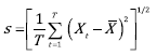 (6)
(6)
where X t represents the condition of the population in each cell at time t (in months). The mean and standard deviation are used for the thresholds to evaluate resilience and stability (see Figure 4B and C and Figure 5B and C).
Resilience R is defined as:
 (7)
(7)
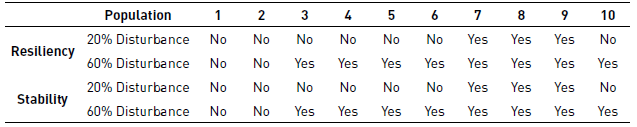
where W t indicates the transition from an unsatisfactory (I) to a satisfactory (S) state:
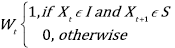
and Z t represents the time that the population (or the hosting cell) remains within the equilibrium range. The subtraction and addition of the standard deviation to the arithmetic average results in the range of cells and population equilibrium. C is the vector that is formed by the dynamics of the population or ecosystem (X t ), the vector (C) being evaluated against the range of ecosystem equilibrium and population equilibrium in each iteration of the model according to the following condition.
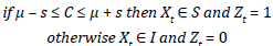
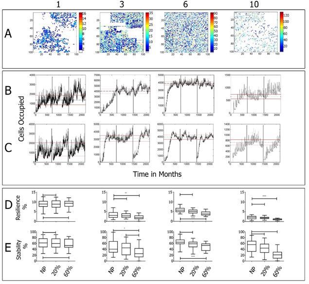
Figure 4 Simulated populations of herbs (1 and 2), a shrub (4) and a tree (10): A) Final spatial distribution of populations (after 180 years); B) Cells occupied by population (dotted line indicates the mean and the solid lines one standard deviation); C) Cells occupied by population after 60% area clearance; D) Resilience index evaluated at baseline, 20% and 60% clearance; E) Stability index for baseline, 20% and 60% clearance.
Stability St (taken as a synonym of reliability, as defined by [63]) is defined as:
 (8)
(8)
The ranges of ecosystem balance and population equilibrium are defined by adding and subtracting the standard deviation to the arithmetic average (μ). Resilience and stability could be evaluated at each point of the time series generated by the model. Z t is satisfactory (S) when the values lie within the range of ecosystem or population at equilibrium, or unsatisfactory (I) otherwise. All values obtained are stored in the vector X t .
3. Results
3.1. Model simulations
We analyze simulations in terms of the spatial development of the populations, identifying patterns that could be similar to those present in real ecosystems. The model ran for the equivalent of 180 years, with each of the simulated populations responding differently to abiotic and biotic conditions (Figure 4A). Each population has features that benefit or deter the ability to settle in a certain cell. Herbs and shrubs tend to show gregarious patterns (with low generational times and high reproductive rates), whereas trees tend to be sparser, lasting longer once established.
Figure 4A shows the spatial distribution of four distinctive populations in the last year of simulation (180 years run total). The patterns observed include “gregarious” clusters (i.e., populations 1 and 3), “overall distribution” pattern (population 6) and “scattered” patterns over cells prone to have good availability of water (population 10). Since the model includes stochastic variables, the results vary among simulations but, in general, populations exhibit similar patterns.
In relation to the behavior of populations over time, Figures 4B and C show the set of simulated populations in time relative to the number of cells occupied for the baseline case (no clearances). After 60 years of simulations, populations stabilize and none of them occupies more than 70% of the cells. The initial part of the series is assumed to be for the establishment stage. The middle section is used to determine the statistics of the established population (mean and standard deviations). In the third part, a scattered clearance of populations is made in 20% (Figure 4B) and 60% (Figure 4C) of the area to compare resilience and stability relative to the baseline case (without clearances).
Figure 5 shows cells occupied by one, three, six and ten populations respectively. The presence of more than two species in the same cell reflects a simulated ecosystem structure under the established biotic and abiotic interactions. The maximum number is reached by cells hosting three and four populations, decreasing gradually in numbers for cells hosting less than three and more than four (See Figure 5 A, B, C, and D). This result shows the rareness of cells hosting all the populations and the common condition of hosting an average number, which is in agreement with “expected” biodiversity conditions in which no cells are likely to host all the populations.
The presence of a certain number of populations in one cell may reflect the structure of the community. At the beginning, it is common to have a high number of cells hosting a single population. That number decays later when more populations start to grow and establish in a succession like phenomenon [67-69], in which the colonization of the first plants with an r strategy occurs until the larger plants became part of the community (see Figures 4B and C). As in the case of the populations, the numbers of cells occupied by different numbers of populations are analyzed in three sections: the time for establishment (first 60 years of the series); the baseline section (second part of the series); and the third part, where a clearance of 20% (Figure 5B) and 60% (Figure 5C) is made.
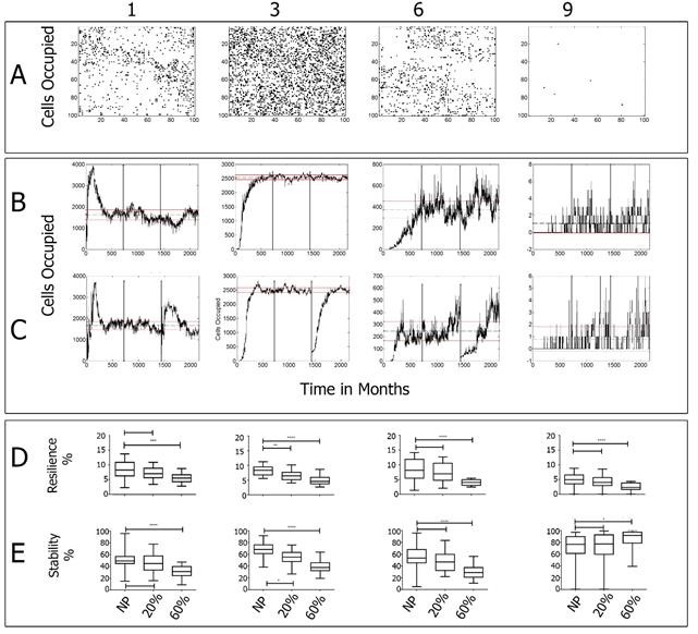
Figure 5 Hosting cells with one, three, six and ten populations; A) Final spatial distribution of populations (after 180 yrs); B) Cells occupied by each population (dotted line indicates the mean, the solid lines one standard deviation); C) Number of cells occupied by one, three, six and nine populations after 60% clearance; D) Resilience index for baseline, 20% and 60% clearance; E) Stability index for baseline, 20% and 60% clearance.
3.2. Resilience and Stability
Initially, we determine the baseline to measure the stability and resilience between 60 and 120 years of simulation. In this period, the populations reach their maximum stability. Both resilience and stability are calculated for each population and for the number of populations inhabiting the same cell with the modified equations.
Subsequently, we measured the stability and resilience for each population, and for the number of populations per cell, after inducing a disturbance. At 120 years of simulation, we applied two area clearances of 20% and 60% of the total area of 100(100 cells. We performed the analysis over thousand simulations. Figure 4C and D show the resiliency and stability of both the baseline and post-disturbance cases for each population. Figure 5C and D show the resiliency and stability results for the number of populations in a cell.
After the clearances, all populations depart from their baseline condition, showing different rates of recovery. Populations with shorter generation times recovered faster (population 1, 2, 3) than populations with longer generation times (population 7, 8, 9, 10) (Figures 4B and C).
For populations in the same cell (Figures 5B and C), there is an increment in the number of cells with one population right after the disturbance due to the loss of ecosystem structure, but gradually the cleared cells gain back the original structure of more than one population per cell. In all cases, the populations tend to occupy the same number of cells as before the perturbation.
From the simulations, it is evident that a 20% clearance is not as disturbing of the ecosystem structure as a 60% clearance. In fact, the departure from equilibrium is barely noticeable in the first case, whereas in the second the structure returns almost to the original stage and requires a recovery time of several years before reaching the stable equilibrium.
3.3 Comparisons of medians for simulated populations
To examine whether there are significant differences in resilience and stability between the simulations at baseline compared with the conditions after 20% and 60% clearances we conducted a multiple comparisons Dunns test. Figures 4 D and E show the result for each population. In general, resiliency and stability decreases slightly with the clearances, being the change more pronounced for the case of a 60% clearance. Populations 1 and 2 (which resemble those of herbaceous plants) are less affected by clearance than the others (see the results for each population in Table 2].
3.4 Comparisons of cells with N populations
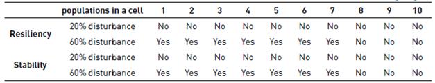
The Dunns test is also used to examine differences in resilience and stability between the simulations at baseline and the conditions after 20% and 60% clearances for cells hosting different numbers of populations [Figures 5D and E). As in the case of the specific populations, the resiliency and stability of hosting cells in the grid decreases with clearances. In this case, the effect is noticeable for all cases, except for cells hosting 9 and 10 populations, since the probability of cells having all populations is low (see the results for number of populations per cell in Table 3].
4. Discussion
Understanding and predicting the variation and persistence of species diversity and community composition in space and time is a central question in ecology [4, 7]. We propose a formal quantification of resilience and stability that shows how disturbances may affect the balance of individuals and communities, identifying a range where resilience and stability may be operating in ecological systems. The ecohydrological model herein presented relates the population behavior of plant species (i.e., plant phenotypes) with natural water availability, temperature, soil conditions and intraspecific and interspecific interactions. These variables are defined in terms of allometric curves. Although arbitrary, the competition rules established in the model (which are based on the concept of ecological niche proposed by Hutchinson [57]) may be operating in real ecosystems and their parameterization brings interesting insights about the way communities may be structured.
The application of allometric and linear rules allows modelling different population phenotypes. The model reproduces different behaviors between populations and survival curves of type I, II, III, or intermediate between them [70]. To apply the rules to a particular population, we review in detail the concept of the n-dimensional hypervolume of species proposed by Hutchinson (1957) [57], considering the limits of tolerance and physiological factors such as competition, reproductive strategy, number of seeds, number of offspring and survival rates. The advantage of the allometric rules is the single requirement of the species weight at the time of their first reproduction to infer all the biological variables of interest in the model. Although in many cases, parameters such as the generation times and life expectancy of natural species are missing or unknown, the weight at the reproduction time may well let to infer the rest of the parameters that affect the ecosystem dynamics.
This model simulates the behavior of populations in a conceptual ecohydrological environment that, nonetheless, could be implemented in a real ecosystem. In this regard, the decisions made by the agent system suggest that the factors that penalize or reward the automatons in each cell could be a good approximation to a real ecosystem. Stochasticity, on one hand, plays an important role in the amount of seeds produced, the survival through germination and the life expectancy of individuals for each population. On the other hand, stochasticity plays a role in the occurrence and distribution of rain and temperature as abiotic factors that are stressors for the populations.
The behavior of agents system, represented by the simulated populations, emerges under all the conditions imposed by the model, such as intra and interspecific competition, and environmental conditions created by the hydrological model. Each population reaches the equilibrium at different times (see Figure 4B), with short times for herbs and long times for trees, but all of them are in equilibrium approximately after 60 years, since the agents (populations) take about that time to "find" their niche and “reach” a relative equilibrium in the number of cells occupied (considering the establishment from zeroes).
Simulated populations show logarithmic growth curves that stabilize in certain carrying capacity (K) and show oscillations in the stable phase. The code does not include the carrying capacity, but rather a seed production rate and survival age. The carrying capacity is the dynamic result of the competition and the space limitations of the simulated area. Therefore, the observed growth curve can be explained as an “emergent property” of populations derived from the model, due to different K for each population. The possibility of calculating K indicates that the observations, conceptualizations, methods and variables can be a good and valid approximation to the theoretical behavior expected in population ecology and may be observed in real populations [55]. The present version of the model does not elucidate the equations for population growth, life tables and fecundity rates, which may be subject of further research.
The functions proposed by Calder [40, 41, 43, 49], that we incorporated in the model, allow the definition of basic features of the population biological structure. While there are exceptions to these rules, they seem to work well in general [71].
Biodiversity, represented in the model as the number of populations in the spatial domain, is a key factor for the recovery of an ecosystem. In this regard, it should be noted that biodiversity can confer resistance to an ecosystem, since a large number of species increase the likelihood of sustaining the processes that occur in an ecosystem in a wider range of conditions, compared to what would do one or few species [4, 72]. That is why the model includes the interaction among different populations, so as to increase their performance and utility [14, 73]. However, there are still limitations to represent biodiversity, since the model does not incorporate, for instance, animal species and their effects for example on pollination for a more realistic representation of an ecosystem.
Although resilience and stability of ecosystems have been pursued theoretically as concepts, there are still no clear methods to measure them [7, 10, 12]. In this regard, our study proposes a method for measuring the resilience and stability of ecosystems through indices that have been adapted and modified from work done initially in hydrology [63]. This is an explicit proposal of how to measure resilience and stability in an ecosystem. Given enough field and remote sensing measurements, the equations proposed in this paper may be adequate at the population and community levels to quantify the recovery time of the ecosystem towards an equilibrium state.
To check the operation of the model, we perform shocks by clearing homogeneous areas from populations. However, the model allows different types of disturbance (for instance, changes in temperature and rainfall regimes, the introduction of new species). It is interesting to observe from the simulations that the behavior of each population and their response to disturbance as a whole follow the logic of the proposed allometric rules and temporal patterns, which largely depends on reproductive rates and strategy type, as suggested by Bohn et al. [52].
On the behavior of populations after a 60 % clearance, species with lower generation times (populations 1 and 2) are not affected by the disruption as the other eight populations where the clearance significantly affects their resilience and stability. With 20% clearance, the perturbation is statistically significant in the resilience and stability only for populations 7, 8 and 9 (corresponding to brushes and trees) but not significant for the other populations (see Table 2). This suggests that the size of the perturbation alters the time of recovery, affecting with more intensity populations with long generation times. No differences are observed in the impact strengths and stabilities relative to baseline for populations 1 and 2, which may be due to their high reproductive rates and capacity of adaptation to these changes. On the other hand, the population 10 does not experience a change in their resilience and stability when subjected to a perturbation of 20% (see Table 2) due to the small number of cells occupied (around 500 cells), which tend to be scattered over the grid.
Table 2 Comparison between unperturbed and perturbed systems in the populations (Yes if differences are statistically significant)
The number of cells with N coexisting populations is a measure of the structural stability of the ecosystem. When subjected to disturbance, In the case of 60 % clearance, all the measurements showed statistical difference, except for the resilience and stability of cells with 8, 9 and 10 cell populations. This is explained by the low probability of 8, 9 or 10 populations coexisting in the same cell. On the other hand, for the 20% clearance there were not statistical differences in any case (see Table 3], indicating that small disturbances may affect the populations but not the overall structure. A problem encountered with the use of equations of resilience and stability is the time scale used to evaluate these properties of ecosystems (180 Years of simulation in this case), since large evaluation times tend to average the statistical differences between a disturbed system and one undisturbed. Therefore, the benchmark to define the time in which they must evaluate the resilience and stability will depend on the generation time of the species of interest.
5. Conclusive remarks
The ecohydrological model introduced in this paper combines a hydrological model with an agent-based system in an effort to quantify the resiliency and stability of ecosystems in the long run, establishing relationships among different plant populations and their environment. The model combines a soil water balance with concepts of current biology to analyze quantitatively the resilience and stability of ecosystems, moving from a conceptual appreciation to a mathematical definition of resilience and stability indices thanks to the modified equations proposed in this article.
These indices become important in times when neotropical terrestrial ecosystems such as the Amazon, mountain and dry - tropical forests are undergoing rapid changes affecting their structure, and when data available and field experiments may be difficult to find in periods of several years, like the ones suggested by the recoveries in our simulations.
The user can modify and adapt the variables in the model to evaluate the resiliency and stability of the assessed ecosystem, provided that sufficient field data for the model parameters are available from real populations in nature.
In this paper we did not consider other methods for examining population abundance (such as life tables, for instance) that can be also used to determine the growth equations for each population. Although other types of disturbances can be incorporated, such as changes in temperature and rainfall under climate change assumptions, our purpose with this first, simple clearance approach was to verify the assumptions and changes occurred given the stability of other factors.
Models such as the one introduced in this paper, which are based on quantitative approaches to the resilience and stability of ecosystems, would be useful for biologists, forest engineers and other environmental professionals to make decisions on restoration and conservation of ecosystems in the long run, especially in tropical forests, faced with climate change scenarios [74].
Future developments of this research will include animal-plant interactions and an evaluation of other perturbations such as trends in precipitation and temperature and more realistic determinations of soil covers, looking for the implementation of data from field measurements and satellite images.

