


 English (pdf)
 Article in xml format
 Article references
 Send this article by e-mail
 Cited by SciELO
  Cited by Google
  Similars in
SciELO
Similars in
SciELO  Similars in Google
 Permalink
1. Introduction
SLAM (Simultaneous Localization and Mapping) builds a map of an unknown environment in an incremental way and uses it for simultaneously estimating the pose of a mobile platform. Along time many variants in the sensor have been presented: sonar rings, laser scanners, perspective cameras, omnidirectional cameras, stereo cameras, inertial sensors, and combination of them. In these systems sparse features such as corners [2], edges [3], or planes [4] have been efficiently used when the camera pose is the primary estimation.
Since the development of cheap and accurate depth sensors, that deliver both depth and RGB images at high frame rates, new systems for dense tracking and mapping in real time have emerged, for example [5,6,7], showing more accurate estimates in camera pose, high quality reconstructions and enabling scene understanding in mobile robotics and more robust augmented reality applications, where an accurate 3D model of a rigid body, updated and expanded in real time, is needed. With this work, we want to extend the possible applications of a dense tracking and mapping system by giving it the ability to detect and localize objects commonly found over desktops, like monitors, laptops, books, cups, and keyboards. An object detection module mounted over a system that tracks and maps the environment using the whole data of the RGB and depth images, can be useful for scene understanding in mobile robotics tasks such as grasping and moving specific objects, dense reconstruction of specific objects using unmanned vehicles that wander in the scene, for object tracking and 3D segmentation, for creating a database with geometric information of instances of an object, for augmented reality using the reconstructed and categorized objects, among others.
Our main contributions are
A modular system for dense tracking and mapping that couples an object detection module for labeling the scene and that can easily be expanded by integrating new modules for manipulating objects, for navigation of unmanned aerial vehicles or for augmented reality.
An algorithm for propagating to the model information of detected objects and for managing multiple instances of an object class, computing its location, a 3D bounding box, and its probability.
A color management algorithm, similar to the truncated signed distance function (TSDF) [8] management, that allows the system to store color information around the whole trajectory and get a model with full color data.
In section 2 we analyze the most important dense SLAM systems that work with depth cameras and outstanding systems for 3D scene labeling. In section 3 we introduce the main modules and describe the general structure of the proposed system. In section 3.1 we focus on the volumetric fusion of partial depth scans. We provide details about the volumetric structure, updates of the TSDFs, the weights, object class data and color data, and about our implementation of marching cubes. Next, in section 3.2 the rasterization process and the model-to-frame ICP is analyzed. In section 3.3 we present some details about the module used for detecting objects (YOLO). In section 3.4 the strategy for differentiating between multiples instances of an object class is described. Our experiments and the results of the performance of the algorithms implemented on a graphic processor are explained in section 4. Finally, we draw our conclusions and future work in section 5.
2. Related work
KinectFusion [5] is the first system that builds a dense reconstruction of room-sized scenes and simultaneously localize the camera at 30Hz, using the Kinect version one, and one GPU. The model-to-frame tracking is based on coarse-to-fine ICP. It minimizes the point-to-plain distance of points matched using projective association rather than feature extraction and matching. The three-level pyramid is built with vertex and normal maps from depth maps coming from the sensor and from the reconstructed model. Once the camera pose is estimated, the depth maps captured with the sensor are fused and the model is updated. The TSDF, is used for storing the depth data through the time, and ray casting for explicitly visualizing the model. Kintinuous [6] based on their previous work [9], is an extension of KinectFusion [5] for working in both room-sized environments and large-scale paths. The cost function integrates the cost of the RGB-D frame-to-frame tracking of [10] (implemented on GPU), and the cost of the original model-to-frame ICP tracking of [5], in order to tackle poor performance when the camera points to a flat wall or corridors with no significant 3D features. They use another visual odometry system called FOVIS [11], that relies on FAST feature correspondences in the RGB images, and that automatically switches when a planar environment appears. Unlike [5], Kintinuous integrates color information, getting full colored models. The color volume is updated based on KinFu [7], but with real time surface coloring and rejection of unreliable color measurements. The next version of Kintinuous [12] includes loop closure with pose-graph optimization and non-rigid space deformation.
ElasticFusion [13] is a map-centric approach that builds a surfel-based map of room-sized environments and tracks the camera with a dense frame-to-model method that combines point-to-plane error and dense photometric error. It performs dense model-to-model local surface loop closures applying a non-rigid space deformation of the map, instead of a standard pose-graph optimization. Global loop closure is achieved with an appearance-based place recognition method. The reconstructed surface is superior to similar systems. ORB-SLAM2 [14] builds globally consistent sparse reconstructions for long-term trajectories with either monocular, stereo or RGB-D inputs, performing in real time on standard CPUs and including loop closure, map reuse and relocalization. This system has three main parallel threads: the tracking with motion only bundle adjustment (BA), the local mapping with local BA, and the loop closing with pose graph optimization and full BA. It does not fuse depth maps but uses ORB features for tracking, mapping and place recognition tasks. With BA and keyframes, it achieves more accuracy in localization than state-of-the-art methods based on ICP or photometric and depth error minimization. Place recognition, based on bag of words, is used for relocalization in case of tracking failure. RGBDTAM [15] combines a semi-dense photometric error (only for pixels belonging to edges) and a dense geometric error (point cloud alignment in a coarse-to-fine scheme with a pyramid of four levels) for camera tracking, achieving CPU real time performance. The tracking thread minimizes the geometric and photometric reprojection error with respect to a previous keyframe. The mapping thread estimates a semi-dense map for every keyframe. The inverse depth is estimated using the raw depth maps from the sensor and multi-view geometry. Bag of words is employed for loop closure and pose-graph optimization over the keyframes for global consistency.
The work [16] labels objects of interest in 3D scenes reconstructed from RGB-D videos. An object detector on the RGB-D frames runs to score individual pixels and then these pixels are projected into the reconstructed 3D scene. The point cloud is voxelized so that each voxel contains a set of 3D points. HOG features are extracted over both the RGB and depth image to capture appearance and shape information of each view of an object. A linear SVM sliding window detector is trained using views of objects from the RGB-D object dataset. These linear score maps are converted into probability maps that define the probability of a point belonging to a certain class. A data term and a pairwise term together define a multi-class pairwise Markov Random Field, whose energy is quickly minimized using graph cuts. The data term measures how well the assigned label fits the observed data and the pairwise term models interactions between adjacent voxels. In this way, local evidence, such as appearance and shape, is combined with dependencies across regions like label smoothness. Lai et al. [17] is a system for scene labeling based on [16] that combines features learned from raw RGB-D images and 3D point clouds directly, without any hand-designed features, to assign an object label to every 3D point in the scene. The data term was computed integrating responses from sliding window detectors on RGB-D frames and responses from the classifier over the 3D voxel data. This approach only requires images containing views of each object in isolation and synthetic 3D models downloaded from an online database on the Web. In [18], a multi-class labeling on a Markov Random Field (MRF) over the voxels of the 3D scene is performed. It does not employ any prior knowledge about the objects to be detected; the set of object classes is previously unknown and needs to be generated online by multi-object hypotheses, unlike [16] that uses pre-learned 2D object models. The results from MRF are further refined by merging the labeled objects, which are spatially connected and have high correlation between color histograms.
Our system tracks a RGB-D camera and builds a dense representation of rom-sized scenes using state-of-the-art algorithms: a model-to-frame tracking with coarse-to-fine ICP and an implicit representation with a volumetric structure that stores TSDF values. Compared with KinectFusion [5], our system does not perform ray casting for getting a depth map from the model but marching cubes and rasterization, taking advantage of the depth buffer available in OpenGL. Other difference with [5] is the color management; we integrate color information sequentially during the reconstruction process similar to Kintinuous [6], but unlike it, our system updates color information of the observed voxels by averaging the accumulated color data with the current one, in a similar way to the update of the TSDF value. Moreover, our system does not use RGB data for tracking (only for coloring the model) and does not perform loop closures with techniques such as space deformation, pose-graph optimization or bundle adjustment, like in [12-15], that makes them more robust to long and complex trajectories. We do not track and reconstruct moving objects like [19,20], but we detect and reconstruct a static desktop-like scene. For labeling the 3d scene, we couple an object detection module YOLO [1] that works in 2D, with the RGB images, instead of working with Random Markov Field that uses features from RGB-D frames as [16] or with RGB-D frames and point clouds as [18]. We can claim that the modular structure of our system enables the easy integration of new modules such as a grasping module with a robotic arm, a path planning module with an unmanned aerial vehicle (UAV) or an augmented reality module.
3. Methodology
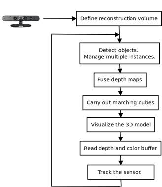
We have implemented a system that constructs a 3D model with either color of the scene or color associated to detected objects, using YOLO detector [1]. The volumetric structure stores in each voxel this color data, information about the surface enclosed by the volume as TSDF values, a weight and object detection data (when YOLO is coupled to the system). The volumetric structure is located (T rcube ) with respect to the initial frame. The depth maps are fused from the estimated poses T wc (using ICP), updating each voxel independently and in parallel, in a graphics processing unit (GPU). After updating the volumetric structure, an explicit representation is computed using an implementation in GPU of marching cubes. We use OpenGL for visualizing the model and for reading the depth and color buffer achieving a predictive depth map and a predictive object detection image from the next camera pose. These images are employed in ICP and multiple instance management. Figure 1 presents the main processes and the structure of the proposed system. In the next sections, the main modules of the system are explained.
3.1 Volumetric fusion
Depth data coming from either a depth camera, a dataset, or built from images obtained with a monocular or stereo camera, must be represented in a global reference frame. A simple representation could be overlapping scans, for example, drawing local point clouds in a global coordinate system. A better representation is obtained with volumetric fusion of depth maps which generates a surface by computing the zero crossing of the function. The surface is represented as a set of triangles in 3D, obtained from the volumetric structure by applying the marching cubes algorithm. This 3D scene is rasterized in a 2D representation in order to visualize it on a screen. This representation is computationally more efficient, more realistic and allows a richer interaction with real or virtual objects, in robotics or augmented reality.
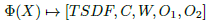
The constituent element of the volumetric structure is a voxel. We will denote a voxel as Φ(X), where X ∈ ℝ 3 is the centroid of the voxel. It stores a TSDF value, a structure with RGB color data C, a weight W, and two structures with object class data O 1 , O 2 , as is shown in Eq. (1).
 (1)
(1)
The TSDF, is a truncated version of the signed distance function (SDF), used in computer graphics for representing surface interfaces as zero, free space as positive values that increases with the distance to the closest surface and (possible) occupied space as a negative value. The structure for color data stores the RGB components of the image coming from the scene, in the range [0,1]. However, if the object detector module is coupled, an image coming from the detector is used instead. The weight reflects the confidence of the TSDF value. Each structure for object class data stores the class identifier and a counter for this class. We use two object class structures: in the first one we store the data of the principal detected object, it means, the object with the greater class counter; in the other one we store the data of the object with the second greater class counter.
Volumetric structure
The user can define the resolution of the reconstructed model through the size of the volumetric structure and the number of voxels in each dimension. The numeration of vertexes and edges of an individual voxel is shown in Figure 2(a). For carrying out marching cubes each vertex must have a TSDF value and a color C. Since each voxel stores just one TSDF and C, we create an extended structure based on the neighboring voxels, as is shown in Figure 2(b).
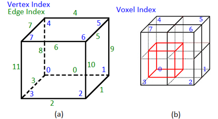
Figure 2 Notation for applying marching cubes. (a) Numeration of edges and vertexes for an individual voxel. (b) Neighboring voxel (in black) used for assigning a TSDF and a color value to each of the eight vertexes of the main voxel (in red)
The TSDF of voxel Φ i (X) is assigned to Vertex i, for i = 0:1:7. The same assignment is done for the RGB color C of the voxel Φ i (X).
Voxel update
The depth measurement D(u), where u=(u,v) is a coordinate in the image plane, has an uncertainty of μ around the true value, so the measure is likely to be in the range [D(u)−μ, D(u) +μ] over the ray that passes through the voxel Φ i (X) (see Figure 3]. The free space is in the range [0, D(u)−μ] and no information about the surface is obtained farther than D(u)+μ (occupied or free space). With TSDF, points that are in free space within a distance greater than μ from the closest surface will be truncated to a maximum value. Points that are far from the visible surface are not measured.
Figure 3 Ray that passes through the voxel i (dark blue), range of uncertainty of the measured depth (yellow), surface been scanned (light blue) and difference between the measured depth and the z-coordinate for a voxel i (in camera frame). The last value is used for computing the TSDF
The TSDF value for a voxel Φ with center X, given the camera pose T wck and a depth map from this pose D ck , is computed using Eq. (2).
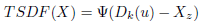 (2)
(2)
where the subindex z corresponds to the z coordinate of the center X of a voxel Φ (referenced to the camera frame) and D k (u) is the depth of the 3D point that lies in the surface and is intersected by the ray. The relation between X and u is defined in Eq. (3).
 (3)
(3)
where π represents perspective projection of the 3D point X = (x,y,z) and dehomogenization by X n (x/z,y/z) and K is the intrinsic camera matrix. Ψ(η) performs the SDF truncation to an argument η(ℝ (see Eq. 2 where η represents the difference of two depths) as is shown in Eq. (4).
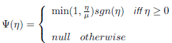 (4)
(4)
The fusion of depth maps in the volumetric structure was formulated according to [8] and [5]. It corresponds to the weighted average of all the TSDF computed with Eq. (5) for each depth map.
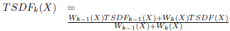 (5)
(5)
where W is the weight of a voxel with centroid X. We propose for color management (see Eq. (6)], motivated by the methodology carried out for updating the TSDF values (see Eq. (5)], the weighted average for each channel of the RGB data through time.
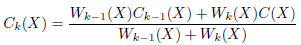 (6)
(6)
where C(X) = I k (u) (RGB image of the scene), and u was defined in (3). If the object detection module is coupled to the system, the color is not obtained directly from the RGB image of the scene, but from a synthetic RGB image I kcod (u), where the color is assigned to each pixel according to the category of detected objects. For example, [1,0,0] (red color) is associated to monitors. If no object is detected, this pixel will have black color. Next, the weight is updated with Eq. (7).
 (7)
(7)
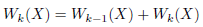
The weight provides information about the uncertainty of a TSDF value, so it can be set according to the depth (directly proportional), and angle between the associated pixel ray direction and the surface normal in the local frame (inversely proportional). However, we used simply W k (X) = 1, that averages the TSDF values, getting good results.
Marching cubes
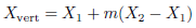
Marching cubes [21] builds an explicit representation given a TSDF volume (polygonal representation of an isosurface of a 3D scalar field). If one vertex is above the isosurface and an adjacent vertex is below, the isosurface cuts the edge between these two vertexes. The position where it cuts the edge will be computed using Eq. (8) by interpolating the TSDF of the adjacent vertexes.
 (8)
(8)
where X vert is the vertex position of a triangle that represents the isosurface, X 1 and X 2 are the position of adjacent vertexes of the cube, with local coordinate system, and m is defined in Eq. (9).
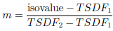 (9)
(9)
with isovalue = 0. The color is interpolated for each channel using the same ratio m (see Eq. (10)].
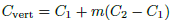 (10)
(10)
We selected marching cubes instead of ray casting [22] for convenience: we already had an efficient implementation of marching cubes in GPU (modified version of the algorithm coming with CUDA). For the additional step of rasterization [23], we simply read the depth buffer from OpenGL (see next section for more details about rasterization).
3.2 Tracking
There are three main frameworks in the literature for dense tracking: frame-to-frame [24] (when a reference depth map is used for aligning locally a synthetic and an observed image), frame-to-model-vertices [5] (the technique that we use and that is explained in the next paragraphs), and frame-to-model-TSDF [25] (a variant of the previous technique that compares values of TSDF instead of vertexes and normals). The goal is to estimate the global camera pose T wck for each new frame where a depth map is available. For using ICP we need to compute at time k a predictive depth map coming from the 3D model updated in time k−1. Next, the computation of the predictive depth map and the ICP algorithm are explained.
Rasterization
This technique [23] is used for displaying 3D models on a screen. A 3D model is represented as a set of triangles. The vertexes of the triangles are projected on a 2D plane (viewer’s monitor), knowing the relative transformation between the model and the camera T cam,model . When a scene is rendered, the information of depth for each pixel is stored in a buffer (see Figure 4]. OpenGL uses it for comparing depth and overriding the depth of the pixel with the depth of the closest object. To take advantage of this buffer, we place the virtual camera on the pose (position and orientation) of the real camera, getting depth information of the scene. No information exists outside the volumetric structure defined by the user for reconstructing it.
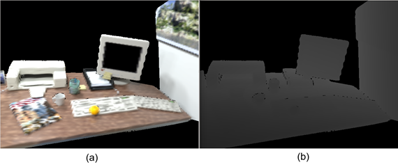
Figure 4 (a) Reconstructed 3D model. (b) Depth map read from the depth buffer of OpenGL. The dark regions correspond to space outside the grid of voxels (no information). The depth buffer is used for frame-model ICP in the tracking process
The frustrum is defined by Z near , Z far and vertical field of view V FOV. The range of depths Z’ stored on the z-buffer is [0,1]. Objects outside the frustrum will not be rendered. After a perspective projection, we obtain Eq. (11).
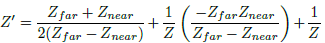 (11)
(11)
where Z is the real depth. Solving for the real depth, we get Eq. (12).
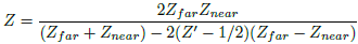 (12)
(12)
We defined Z near as the focal length (in metric units), Z far = 100m and the vertical field of view is computed using Eq. (13).
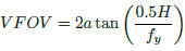 (13)
(13)
where H is the number of rows of the image.
Dense ICP
Dense ICP is appropriate due to two reasons. First, the camera motion at frame rate is small, so we can use fast projective data association to obtain correspondence and point plane metric [5] for pose optimization. Second, these algorithms are highly parallelizable so an important speed up is obtained when implemented on GPU. The general diagram of the frame-model tracking is shown in Figure 5.
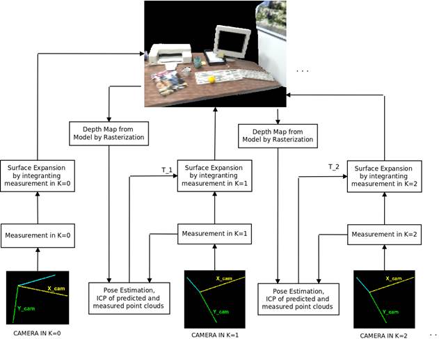
Figure 5 Diagram of the frame-model based tracking. The vertex map in k−1, obtained from z-buffer of OpenGL, is aligned (ICP) with the vertex map, computed from the measured depth map in k
For each depth map, whether estimated from the model,  , or acquired from the sensor, Dk(u), we compute a vertex map and a normal map,
  ,
,  and V
k
(u), N
k
(u), respectively. The vertex map is computed with Eq. (14).
and V
k
(u), N
k
(u), respectively. The vertex map is computed with Eq. (14).
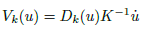 (14)
(14)
and the normal map is computed with Eq. (15) as the cross product between two vectors obtained from the neighbors of the current vertex u.
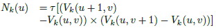 (15)
(15)
where the dot over a vector denotes homogeneous vector and  , it means, a unit normal vector. The transformation from a local coordinate system to a global one is defined in Eq. (16).
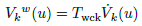 (16)
(16)
Energy Function
Eq. (17) is a global point-to-plane energy, that uses global coordinates for vertexes and normals, and a L2 norm of the error, having as argument to minimize the transformation T wck .
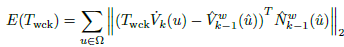 (17)
(17)
This energy aligns, using Levenberg-Marquardt, a live surface (V
k
, N
k
) with a predicted surface from the model in the previous step  by penalizing long distances between the vertex V
k
and the tangent plane to vertex
by penalizing long distances between the vertex V
k
and the tangent plane to vertex (see Figure 6].
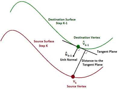
Figure 6 Graphical interpretation of the point-to-plane optimization. The vertex V k (in red), obtained from the measurement, is moved in order to reduce the distance to the tangent plane of vertex Vˆ k−1 obtained from the model
The correspondences are computed by projecting the vertexes obtained from the range sensor in time k to the image plane of camera in time k − 1, using an estimate for the frame-frame transformation 
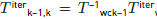 , defined in Eq. (18).
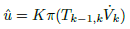 (18)
(18)
Transformation update
We initialize the iterative optimization with T 0 wck =T wck−1 . The global camera transformation is updated, assuming a small change in position and orientation, by pre-multiplying an incremental transformation to the current estimate, as is shown in Eq. (19).
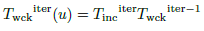 (19)
(19)
where T inc iter is defined in Eq. (20).
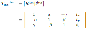 (20)
(20)
This rigid body transformation can be written as a 6-elements vector, as is expressed in Eq. (21).
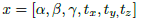 (21)
(21)
With this new transformation, a new vertex map, that reduces the alignment error, is computed through Eq. (22).
 (22)
(22)
Expressing it using the motion vector x (see Eq. (21)] we get Eq. (23).
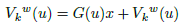 (23)
(23)
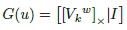
where G(u) consist of the skew-symmetric representation of V k w and a 3×3 identity matrix, as is defined in Eq. (24).
 (24)
(24)
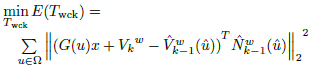
The energy of a linearized version of Eq. (17) can be expressed in terms of the motion vector x, resulting the minimization problem of Eq. (25).
 (25)
(25)
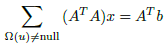
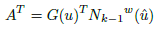
Deriving the objective function with respect to the motion vector x and setting to 0, a symmetric linear system of 6×6, for each correspondence, is obtained (see Eq. (26), (27) and (28), and the paper [5] for more details).
 (26)
(26)
 (27)
(27)
 (28)
(28)
We need a coarse-to-fine scheme since the point-plane error function is linearized, otherwise just small motions can be estimated. In this sense, we built a 3-level pyramid, with a scale of 0.5 between levels (coarsest image of 160x120 pixels). The data association based on perspective projection and the optimization based on the point-to-plane metric is performed in each level, and the result in the coarsest level is used as initial value in the iterative optimization on the following finest level, using Levenberg-Marquardt. With this scheme, we achieve better estimations when fast camera motion occurs and a faster convergence in the finest level (image of 640x480 pixels) since an approximated camera pose has already been estimated in coarser levels (see experiments in [26] for more details about convergence with a coarse-to-fine scheme).
3.3 Object detection
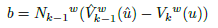
We couple YOLO (you only look once) [1] to our system for object detection in real time. YOLO can detect over 9000 object categories, achieving 78.6 mAP at 40FPS (running on a Geforce GTX Titan X). It applies a single neural network to the full image. This network divides the image into regions and predicts bounding boxes and probabilities for each region. This makes it extremely fast, more than 1000x faster than R-CNN and 100x faster than Fast R-CNN. The model, called Darknet-19 [27], has 19 convolutional layers and 5 maxpooling layers. Moreover, YOLO uses WordTree to combine multiple datasets together in a sensible fashion. YOLO9000 learns to find objects in images using the detection data in COCO and it learns to classify a wide variety of these objects using data from ImageNet [28]. The model only uses convolutional and pooling layers which makes it robust to running on images of different sizes. Figure 7(a) shows the output from the object detector YOLO. A color is associated to the detections that have a probability higher than 50% and belong to any of these five categories: computer, laptop, keyboard, book and cup. Figure 7(b) shows the resulting image, I cod (u), which is used in the color update process, carried out in parallel for each voxel. A pixel with depth greater than the mean depth of the pixels inside the associated edging box is set to black.
3.4 Multiple instance management
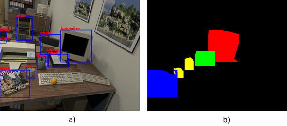
The system can differentiate between multiple instances of the same class that are in the reconstructed model. For achieving that, we read the color buffer of OpenGL that represents the 3D-2D projection of the 3D model, updated until time step k−1, in the image plane located in the estimated camera pose in time step k, it means, we predict where the objects will be found in the next step. Then, we compare the predicted image  [Figure 8(a)) with the image obtained from the object detection module
  [Figure 8(b)).
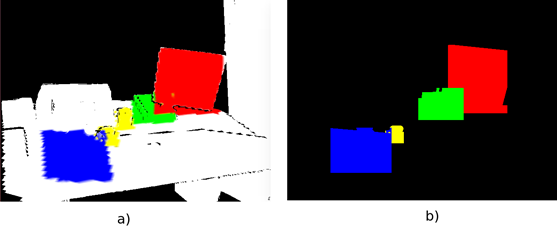
Figure 8 Images used for managing multiple instances of object classes. (a) shows the predicted object detection image, Iˆ cod (u), coming from the model by reading the color buffer of OpenGL. (b) shows the object detection image I cod (u) coming from YOLO
We save information of the objects found in the scene in a vector: coordinates of the 3D edging box, centroid, and identifier. According to whether an object has been detected previously or is a new detection, on an empty or busy region, the object is included in the vector of found objects or the information of an existing object is updated. Figure 9 describes the multiple instance management process.
4. Results and discussion
Our system for dense tracking and mapping, with color from the scene or from the object detection module, runs on a laptop ASUS G551VW with a processor Intel Core i7-2.6GHz, 8GB of RAM memory, a graphics processor NVIDIA GEFORCE 960M and Ubuntu 14.04 as operating system. We carried out experiments with three sequences from the TUM RGB-D dataset [29] that provides color and depth images of a Kinect sensor, with camera pose estimated with a high-accuracy motion-capture system. We also use both a synthetic dataset of Handa et al. [30] which provides the ground truth in camera pose (perfect ray-traced images taken at 100fps) and our own data coming from a Kinect sensor moved by hand in a room-sized scene. OpenCV is employed for processing images, Eigen3 for some matrix operations, OpenGL for drawing the 3D model, and for getting depth and color information from the model, Cuda 7.5 and Thrust library for improving the performance using commodity graphics hardware, YOLO for detecting objects in a desktop-like environment, and OpenNI for working with the Kinect.
Experiments are made for computing the accuracy of the tracking algorithm, the accuracy of the reconstructed 3D model and the performance of the object detection module. We will also evaluate the performance of the main components of the system with respect to time.
4.1 Accuracy in camera pose
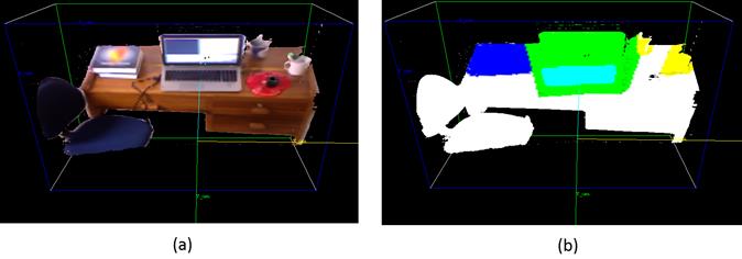
For these experiments, we use the synthetic and the TUM RGB-D dataset. For the synthetic one, the voxel grid has 128×128×128 voxels in each dimension, covering a volume of 1.8×1.5×1m. The volumetric structure is placed using as reference the first coordinate frame of the camera (initialized by the user). Its location is (−1.2m, −0.8m, 0.7m). The final reconstruction has 788,373 vertexes. Figure 10(a) shows the resulting 3D reconstruction with data coming from the scene. Figure 10(b) shows the same reconstruction but using color coming from the object detection module. Neither the geometry of the 3D model nor the estimation of the camera pose is affected by the type of color used.
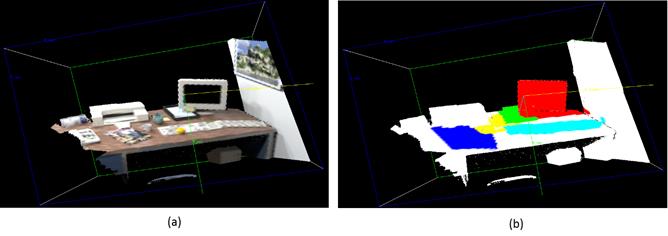
Figure 10 Resulting 3D reconstruction with color (a) from the scene and (b) from the object detector. Synthetic depth maps are fused from the estimated camera poses
The maximum number of iterations for camera tracking in each level is 4,8,10, from fine to coarse level. We define the error in camera position as the Euclidean distance between the ground truth and the estimations. The behavior of the error in camera position around the whole trajectory is shown in Figure 11.
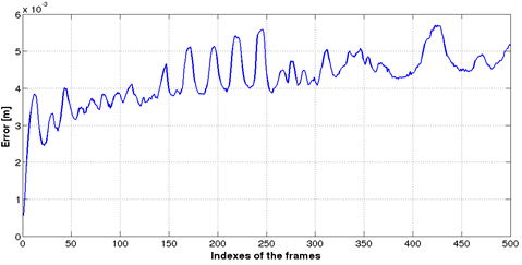
Figure 11 Error in camera position for synthetic data. The error remains small without drift after completing the whole trajectory
The analysis in orientation is made in each axis, as the difference between the ground truth and the estimated values. These errors are shown in Figure 12.
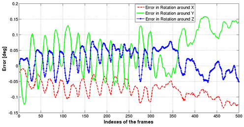
Figure 12 Error in camera rotation for synthetic data. The error remains small without drift after completing the whole trajectory
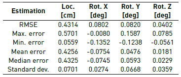
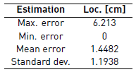
Table 1 summarizes the quantization of the errors in camera position and orientation. Note that the root mean square error RMSE in camera position (less than 1cm) and in camera orientation (less than one tenth of a degree) shows the high accuracy of the tracking algorithm. Moreover, the error in camera position remains stable after 500 iterations which indicates that no large drift occurs in camera tracking. The RMSE in camera position is 0.59% of the distance navigated by the camera that corresponds to 7.27m.
For the TUM RGB-D dataset, se chose three sequences that were taken in room-sized environments, the fr1/desk, fr1/desk2 and fr1/xyz. For the first sequence (similar configuration for the remaining two sequences), the voxel grid has 128×128×128 voxels, covering a volume of 3×2×3m. The volumetric structure is placed in (−2.5m, −1.1m, 0.3m) with respect to the first coordinate frame of the camera. The final reconstruction has 763,086 vertexes. The maximum number of iterations for camera tracking in each level is 4,8,10, from fine to coarse level. Figure 13 shows the resulting 3D reconstruction with data coming from the scene.
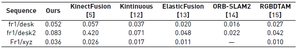
In Table 2 we can see that KinectFusion [5] and our system has similar accuracy (except for fr1/desk2 where [5] has a high error). It is due to similarities in the design: dense ICP for tracking and volumetric structure with TSDF values for the model. More recent systems [12-15], use both photometric and geometric error for estimating the camera pose. Moreover, they include modules for achieving loop closure detection and global consistency with techniques such as non-rigid deformation, pose-graph optimization and bundle adjustment. These systems are more accurate and robust than [5] and our system, especially when performing in complex trajectories (see Table 2]. Note that ORB-SLAM2 [14] is the most accurate system for tracking.
4.2 Accuracy in 3D geometry
The error in 3D geometry is computed by comparing a triangular mesh from a loaded model and the point cloud made up of vertexes of the reconstructed model. We use a 3D model that represents a desktop-like environment, downloaded from TurboSquid, and the software CloudCompare for performing the comparison. The 3D model is loaded in OpenGL, using just geometric data [Figure 14(a)). The virtual camera is located in such a way that circular and vertical scanning at different longitudes (changes in azimuth and elevation of 10o) are performed. The optical axis of the virtual camera is always pointing to the origin that coincides with the centroid of the loaded model. Depth images, obtained by reading the depth buffer from OpenGL, are fused into a volumetric structure. The vertexes of the triangular mesh, computed with marching cubes, are used for the comparison [Figure 14(b)).
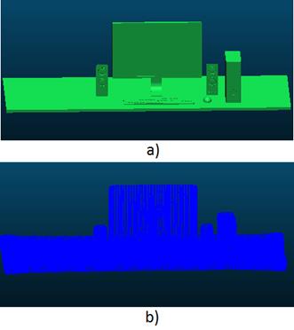
Figure 14 Data used for quantifying the accuracy in geometry. a) 3D Model of a desktop-like environment. Downloaded from TurboSquid. b) Point cloud from the reconstruction
Figure 15 shows the resulting comparison as a point cloud with color representing the error. Note that the greater errors are in the farther edges of the desk. Table 3 summarizes this comparison.
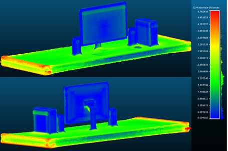
Figure 15 Point Cloud (front and back views) with color representing the distance between the point cloud and the reference model (scale in centimeters)
4.3 Assessment of the object detection module
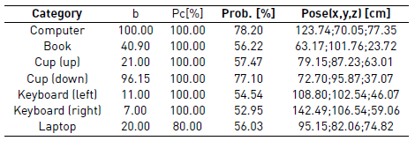
We work with five categories of objects commonly found in desktop-like environments, detected with a probability higher than 50%. Table 4 summarizes the performance of the object detection module using the dataset of Handa et al. [30] (see Figure 10]. Pt is the percentage of detections with respect to the total amount of images where the object is visible. Pc is the percentage of correct detections with respect to the total amount of detections. The pose of each object with respect to the closest upper left corner of the volumetric structure are presented in the fifth column. The computer and cup (down) are detected in all and almost all the images where the objects are visible, respectively. The keyboards are the objects less detected. Wrong detections only occur for the laptop, which sometimes is labeled as book (although this object is really a shelf for leaves and not a laptop). In the last case, where the same object has labeled with two different categories (laptop and book), the system propagates the color to the volumetric structure if the identifier corresponds to the object with greater counter. Otherwise, the counter of the auxiliary object (Object2) is increased but the color is not propagated, reducing instability in the color of the structure. Note that the algorithm in Figure 9 allows the system to manage two instances of cup and keyboard, saving the centroid (pose in Table 4] and 3D edging boxes.
4.4 Time
All the main processes that make up the proposed system were implemented on commodity graphics hardware. Table 5 shows the average on processing time for marching cubes, fusion of depth maps, rasterization, and tracking of the depth camera.
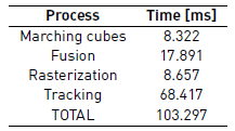
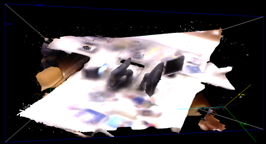
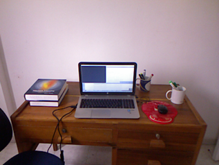
With this performance, the system can reconstruct the scene and estimate the camera pose at 10 fps. Note that tracking is the process with more time consumption. It works with three pyramid levels and {10,8,4} iterations, from coarse to fine levels. The improvement with respect to time of the tracking algorithm is left for future work. The object detection module runs offline, taking 140 ms for processing an image. We saved the information of detected objects in a text file. This file is used in the reconstruction process for creating the image I cod (u) which is propagated to the volumetric structure. Figure 16 shows a real desktop-like environment, taken with the Kinect, while Figure 17(a) presents the 3D model. Figure 17(b) shows the same model but with color representing the detected objects (books, laptop, keyboard and cups).
5. Conclusions
We have developed a system that creates a dense reconstruction of a desktop-like environment and simultaneously estimates the pose of a depth camera moved by hand. All the data of the images is used, depth data for tracking and intensity data for coloring the model, so the implementation was done in commodity graphics hardware, achieving to fuse depth maps and track the camera at 10 fps, with color information. We also couple an object detector and propagate the detections to the volumetric structure in a straight way, saving data of detected objects around the time, managing multiple instances and achieving stability in the color of the model. The results have been satisfactory. First, the ICP algorithm with a coarse to fine scheme, fusion and marching cubes algorithms, produce high accuracy estimates in both camera tracking (especially with the synthetic dataset) and 3D reconstruction. For the experiment with synthetic dataset, the RMSE is 0.431cm in translation (just 0.59% of the distance navigated by the camera) and 0.080o, 0.082o, and 0.040o, in rotation around the X, Y, and Z axis, respectively. For the experiment with the TUM RGB-D dataset, we got 5.2cm, 8.3cm and 3.6cm for translation RMSE. The accuracy of our system is on par with [5] but lower than systems such as [12-15] that integrate techniques for achieving global consistency such as appearance-based place recognition for loop closure detection, non-rigid space deformation, pose-graph optimization and bundle adjustment. Second, the system updates the color of the model every frame, getting a 3D model with color coming from the scene or with color coming from the object detection module. The assessment in geometry of the reconstruction got for the loaded model of Figure 14.a, shows that the mean error is 1.4482cm, less than 1%, considering that the model has 2m long. Third, the system can manage multiple instances of an object class and wrong detections, getting a stable color model. For future work we will integrate the RGB data in the error function for tracking the sensor and implement techniques for loop closure and global consistency that makes the system more robust to complex trajectories. Moreover, we will work on the segmentation of the detected object inside the edging box in order to propagate a more accurate information to the volumetric structure, and on the improvement of the tracking algorithm with respect to time.

