Inglés (pdf)
 Articulo en XML
 Referencias del artículo
 Enviar articulo por email
 Citado por SciELO
  Citado por Google
  Similares en
SciELO
Similares en
SciELO  Similares en Google
 Permalink
1. Introduction
The development of reliable and powerful process simulators, with good databases and ease of communication is mainly carried out by private and foreign enterprises. Such companies put simulators on the market at higher prices, and most of the times, inaccessible for mid-range and small-range domestic enterprises, public higher education institutions, and new research groups. The EMSO (Environment for Modeling, Simulation, and Optimization) can be considered as a good option among those of free access (e.g. COCO simulator, Ascend, etc.) and it has been developed as free software by the ALSOC Project, which is financed by the Brazilian Government and certain private and public institutions. Several publications validate the growing importance of the EMSO software [1-6]. This simulator is a graphical environment where the user can easily carry out the tasks of modeling, simulation, optimization, parameter estimation, and data reconciliation, among others. The software allows both the development of code-based models and the development of models composed graphically by connecting several built-in models from the EMSO Model Library (EML) or those created previously by the users themselves. A previous work shows the application and the advantages of using EMSO as a computational tool for assisting a course of chemical engineering reactions [7]. In addition, EMSO allows data communication with other software and/or devices, such as MATLAB® and Scilab® (free use), by means of external interfaces like the EMSO-MATLAB-SCILAB [8]. Another advantage of this software is the possibility of communicating with other devices such as the PLC (Programmable Logic Controller) via OPC communication and an interface called EMSO-OPC. OPC (stands for Object Linking and Embedding for Process Control) makes reference to a communication standard in the field of control and supervision of industrial processes. It is based on a Microsoft® technology that has a common interface for communication to allow standalone software components to interact and share data. OPC communication is done through client-server architecture. The OPC server is the data source (like a hardware device located in the plant) and any application compatible with OPC communication can have access to the server in order to read/write any variable available within it. This approach is an open and flexible solution to the classic problem of proprietary drivers. Practically all major developers of control systems, instrumentation and processes have included OPC in their products. The present work illustrates the procedure for the modeling and control of a process by using the EMSO simulator and a SIMATIC S7-200 PLC as an OPC communication interface. This document is organized as follows:
Section 2 describes the methodology used for obtaining the phenomenological-based models and the implementation of control systems via OPC. Section 3 describes the statement of a Phenomenological-Based Semiphysical Model (PBSM), estimation of unknown parameters, the validation of the model obtained and the implementation of control systems using EMSO. Finally, section 4 gives the conclusions of the paper.
2. Methodology
2.1 Equipment and Instrumentation
The following resources were used in the development of this project:
(1). a control laboratory module for level and flow control,
(2). a SIMATIC S7-200 Programmable Logic Controller (PLC),
(3). a TCP/IP connection cable,
(4). a laptop computer,
(5). the EMSO simulator and its OPC interface, EMSO-OPC, and
(6). Siemens S7-200 PC-Access software (needed for setting up an OPC server using the PLC controller).
The methodology of the current work can be divided into two fundamental stages: (1) the process model statement and (2) the process control via OPC communication.
2.2 Process model statement
In this paper, the methodology proposed by Álvarez et al. [9] is used to obtain Phenomenological-Based Semiphysical Models (PBSM) by using empirical correlations and basic process principles of mass, energy and momentum balances. The main steps proposed by the authors are listed below, which were followed for process modeling in this work:
Write a verbal description and draw a process flow diagram for the process to be studied.
Fix a level of detail to be used in the model.
Define many process systems (PS) over the whole process to be modeled as required by the level of detail specified in the previous step and sketch a block diagram showing the different process systems and its interactions.
Apply the conservation principles of mass, energy and momentum over each process system.
From the conservation principles, select those balance dynamic Equations (BDE) with relevance to accomplish the objective of the model.
Define the known parameters, variables and constants for the relevant BDEs in each process system.
Find constitutive Equations for computing many parameters as possible in each process system.
Check the degrees of freedom of the model.
Obtain the computational model or model solution.
Validate the model under different conditions to assess its performance.
The modeling method described by the aforementioned authors was carried out to develop a mathematical model for a laboratory process module to control level and flow. The system modeling, the parameter estimation and model validation were done using the EMSO simulator as described in sections 3.1 and 3.2.
2.3 Process Control via OPC communication
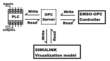
With the aim of designing and analyzing the behavior of different control systems implemented in a process via OPC, mathematical models were developed for PID and PBSM-Based controllers. This was done to establish a clear and concise methodology to implement control and supervision systems in process modules by using the EMSO-OPC application. Firstly, it is worth mentioning that although the EMSO-OPC application allows the implementation of control systems via OPC using models written in the EMSO modeling language, it does not (currently) offer any capabilities to plot the response of process variables (supervision). Therefore, an additional OPC-based application is required to plot the results. In the present work, the software SIMULINK (from MATLAB) was used as an OPC client for the reading and visualization of the process variables. In addition, a SIMATIC S7-200 PLC was employed as an interface for OPC communication between the process instrumentation and the mathematical computing model of the control system. Figure 1 shows a diagram of the connections used in the laboratory.
The different steps for obtaining and implementing a control system using EMSO and EMSO-OPC are described below. In order to illustrate the procedure used, a case study that implements a model-based control over a flow module was considered, including the following stages:
Create a mathematical model for the process controller.
Configure the OPC server.
Set the connection between the variables of the EMSO model and variables of the OPC server.
Create an OPC client application to visualize the process variables via OPC connection.
Implement the control system start up the process.
The methodology described was carried out to implement two different controllers for the studied process module. Section 3.3 shows the detailed implementation of the process control system.
3. Results
3.1 Modeling of a laboratory module for controlling flow and level
The Flow Control Module (see Figure 2] basically involves a piping system connected to two interacting tanks that are filled with water and then emptied in order to analyze and/or control the tank filling process. The module contains the following process elements: two gas cylinders (TK-01 y TK-02), an orifice plate (FE-01), an U-tube manometer (PDI-01), a flow switch (FS-01), a flow transmitter (FT-01), three differential pressure cells (LT-01 to LT-03), two level gauge indicators (LGI-01 y LGI-02), two pressure-current transducers (LY-01 and FY-01), two current-pressure transducers (LY-02 and FY-02), four pressure gauge indicators (PI-01 to PI-04), a pneumatic control valve (LCV-01), an electric-actuated control valve (LCV-02), two centrifugal pumps (P-01 and P-02), a recycling tank (TK-03), two PID controllers (LIC-01 and FIC-02), and several manual valves (V-01 to V-23) to interact with the flow directions in the whole system.
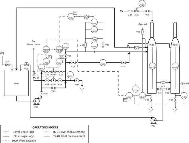
The process module described can be set to different operational modes for filling and draining of the tanks, depending on the configuration adopted for the valves V-19 to V-22 (valves V-20, V-21, and V22 are also referred as VF3, VF4, and VF5, respectively, in Equations (8) -(10) of the process model). In total, the module can be set in 16 different ways, but if the systems with the pressurization valve (V-19) are omitted, the total number of operational modes can be reduced to the following 9:
1). Use of tank TK-01 only and considering gravity discharge.
2). Use of tanks TK-01 and TK-02 with gravity discharge through the TK-01 discharge.
3). Use of tanks TK-01 and TK-02 with gravity discharge through the TK-02 discharge.
4). Use of tanks TK-01 and TK-02 with gravity discharge through both discharges.
5). Use of tank TK-01 with pumping discharge.
6). Use of tanks TK-01 and TK-02 with pumping discharge through the TK-01 discharge.
7). Use of tanks TK-01 and TK-02 with pumping discharge through the TK-02 discharge.
8). Use of tanks TK-01 and TK-02 with pumping discharge through the both discharges.
Several control systems can be implemented in the system studied in order to control level and/or flow. The following control schemes can be mentioned as example: (1) a single loop for controlling the tank level, (2) a single loop for controlling the input flow, and (3) a cascade control scheme for controlling the tank level by using the input flow as a secondary variable, as shown in Figure 2. However, if the possibility of connecting the process module to a data acquisition system and a computer via OPC communication is considered, additional advanced control strategies can be tested.
The proposed model aims to answer the question: how does the liquid level inside the tanks vary when subjected to disturbances such as changes in the feed flow or in the discharge flow? In order to answer this question, a macroscopic scale model (lumped parameters) is used and described by ordinary differential Equations. Figure 3 shows a block flow diagram for the different process systems (PS) considered for the model deduction and the interactions between them.
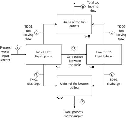
The model to be developed is of macroscopic scale. Therefore, the only process systems considered are the different compartments between the tanks: Systems I and II consist of the liquid phases in the tanks TK-01 and TK-02, respectively. System III represents the connection among the discharges of the two tanks.
In order to accomplish the model objectives, the balances of mass and energy for each process system must be stated. The following assumptions were considered in the deduction of the model:
Properties of liquids are considered constant in each of the process systems considered (lumped parameters).
Frictional and accessory losses are considered negligible.
All the processes are considered isothermal.
The operating volumes of the liquid phases are always inside the cylindrical section of the tanks.
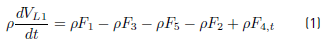
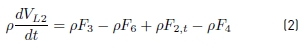
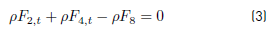
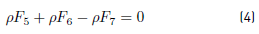
By applying the conservation principle to the process systems shown in Figure 3, the PBSM model is obtained using Equations (1)-(5):
Liquid level in tank TK-01 (System S-I):
Liquid level in tank TK-02 (System S-II):
Total top stream flow leaving the system (System S-III):
Total bottom stream flow leaving the system (System S-IV):
Balance of mechanical energy in the system (System S-IV):
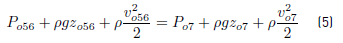
Where, the subscript o56 refers to the joining points in the tank discharges and the subscript o7 refers to the final discharge to TK-03. The rest of the subscripts are used to refer to the numbers of the different streams shown in Figure 3.
Equations (1) and (2) correspond to the dynamics of the liquid volumes inside the Systems I and II, respectively; and solving them, the values of the levels (L1 and L2) we are interested in can be found. Although the remaining Equations are stated in steady-state, they are needed to compute the aforementioned variables.
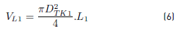
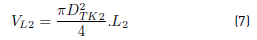
Equations (1)-(5) establish the phenomenological basis of the model for tanks TK-01 and TK-02. In order to solve them, the following constitutive Equations need to be stated: Equations [6-7] for calculating the operating liquid volumes inside the tanks (VL1, VL2), Equations (8)-(10) for calculating the discharge flows (F3, F5, F6) and Equations (13-16) for calculating the top stream flows transferred between the tanks (F2,t and F4,t).
The model stated here is used for predicting the levels inside the tanks. Apart from the physical properties of the liquids and the geometrical parameters of the tanks, the other variables and parameters that must be specified, estimated, or computed using constitutive Equations, are:
Operating liquid volumes
Discharge flows of the tanks:
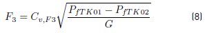
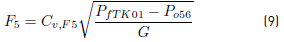
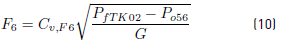
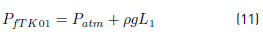
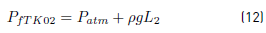
Where, the pressures at the bottom of the tanks are given by Equations [(11), (12)]:
Top stream flows leaving the tanks
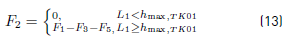
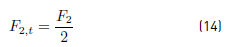
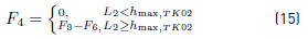
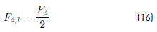
Where  and F 2,t denote the flows entering to one tank from the other in case of tank overfilling, which can be approximated by Equations (14) and (16) when having a flow through equal diameter pipes and neglecting the flow resistance.
The flow velocity for the final discharge can be approximated as in Equation (17):
The Equations system that needs to be solved is given by Equations (1)-(17). An analysis of the degrees of freedom for this model shows that if the input flow (F1) is specified, the values of the coefficients CV,F3, CV,F5 and CV,F6 for simulating the model have to be known. In order to estimate the values of such coefficients, several parameter estimation procedures must be carried out, as shown in section 3.2.
3.2 Parameter estimation and model validation
The following experiments were carried out in order estimate the unknown parameters:
1). Draining of tank TK-01 using the discharge pump.
2). Draining of tank TK-01 by gravity discharge.
3). “Opening vs. Volumetric Flow” curve of the pneumatic valve.
4). Calibration curve of the differential pressure cell used for measuring the level in tank TK-02.
5). Draining of tank TK-02 by gravity discharge.
6). Draining of tank TK-01 towards tank TK-02.
7). Filling of tank TK-01 with gravity discharge.
8). Filling of tanks TK-01 and TK-02 with gravity discharge through the outlet of the first tank.
9). Filling of tanks TK-01 and TK-02 with gravity discharge through the outlet of the second tank.
10). Filling of tanks TK-01 and TK-02 with gravity discharge through the outlets of both tanks.
Initially, experiments 1, 2, 5, and 6 were performed in order to estimate the parameters of each subsystem separately. Experiment 1 was used to estimate the total discharge flow when using the discharge pump. Experiments 2 and 5 were used to estimate the apparent flow coefficients of the valves located at the discharges of tanks TK-01 and TK-02, respectively. Experiment 6 was used to estimate the apparent flow coefficient of the discharge valve located at the point of interconnection between tanks TK-01 and TK-02. The discharge flow when using the discharge pump was determined experimentally to be about 44.94 l/min. This result was obtained by measuring the time taken for the level to go down between two specific points of the level indicator tape.
Experiment 7 was performed in order to estimate the apparent flow coefficient of the discharge valve located at tank TK-01 while the tank is both filled and drained by gravity.
Performing experiments 8 to 10 allowed estimating the different valve coefficients from the values initially estimated in the separate analyses of each subsystem. Figures 4 and 5 show the level dynamics observed experimentally (see white markers), the level dynamics given by the model (see continuous lines), and the experimental data used in the model validation (see black markers) for the variables L1 and L2, in the different operating modes considered. The values of the estimated parameters of all the operating modes are summarized in Table 1.
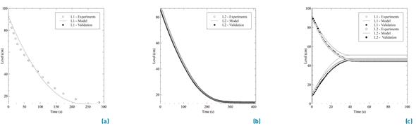
Figure 4 a) Level dynamics when draining tank TK-01 by gravity, b) level dynamics when draining tank TK-02 by gravity, and c) level dynamics when draining tank TK-01 by gravity towards the tank TK-02
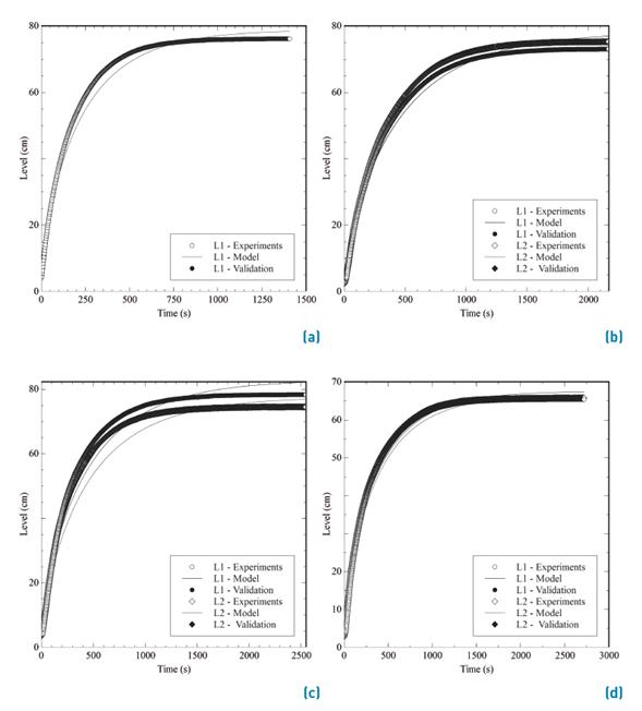
Figure 5 a) Level dynamics when filling tank TK-01 with gravity discharge, b) level dynamics when filling the tanks TK-01 and TK-02 with discharge through the outlet of TK-01, c) level dynamics when filling tanks TK-01 and TK-02 with discharge through the outlet of TK-02, and d) level dynamics when filling tanks TK-01 and TK-02 with discharge through the outlet of both tanks
As can be seen in Figure 4 and 5, the model offers very good predictions of the actual system. Although the model predictions (see continuous line) show a certain degree of deviation from the experimental data (see markers), it is clear that the major deviations were obtained for the separate analyses of the subsystems and not in the dynamical analyses. In general, the model predicts well the qualitative and quantitative behaviors observed in the actual system.
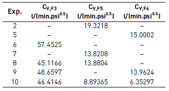
From Table 1, it is evident that the results obtained separately showed different values for the estimated parameters. This indicates that the parameters vary when the operating mode of the process system changes from one operating mode to another. Hence, there is not a unique set of universal parameters for all the operating modes as expected in a steady-state flow through a valve. However, it can be seen that when the valves interact, as in experiments 8 to 10, the process dynamics set the valve coefficients values in order to assure the mass and energy balances for each specific dynamic.
3.3 Implementation of control systems using EMSO
Creating the controller mathematical model
A simulable mathematical model or FlowSheet (with file extension *.mso) must be created in EMSO. This FlowSheet must contain among its specifications (the SPECIFY section) the input variables referring to the read signals from the OPC server [10,11].
OPC Server configuration
In order to read and/or write data from/to an OPC server using a PLC as an interface, a configuration file is required to allow the access to the desired variables in the server. In the case of the SIMATIC S7-200 PLC controller, this file has the extension *.pca and contains the names, the data types, and the memory addresses of all the PLC variables required to create the OPC server. The basic procedure for the setting up an OPC server with the SIMATIC S7-200 PLC is described in [12].
Setting the connection between the EMSO model and the OPC server
A file (with extension *.eof) must be created using the EMSO-OPC application to set up the OPC connection between the EMSO model file (extension *.mso) and the OPC server. All the connections between the EMSO model variables and the OPC server tags must be listed in that file. Figure 6 shows the graphical user interface of the EMSO-OPC application and some connection examples.
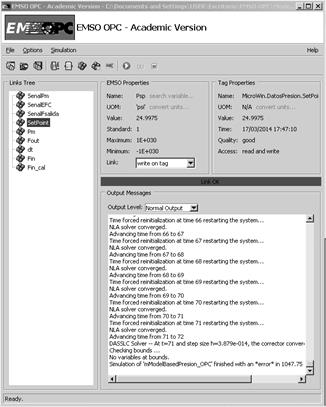
The basic procedure for configuring the OPC connections among the EMSO model variables and the OPC server tag is as follows:
1). Create a new EMSO-OPC Project.
2). Select the OPC server you want to work with.
3). Select the simulable mathematical model (FlowSheet entity) of the controller.
4). Create the links or connections by searching the respective EMSO model variables and OPC server tags you want to connect. It is important to specify whether the OPC server tag in each link is read-only (Read from tag) or write-only (Write on tag).
5). It is important to check that the OPC server tags can be read correctly before proceeding. Otherwise, check that the data types on the OPC server correspond to DINT or REAL data types.
Creating an application for visualizing the process variables via OPC
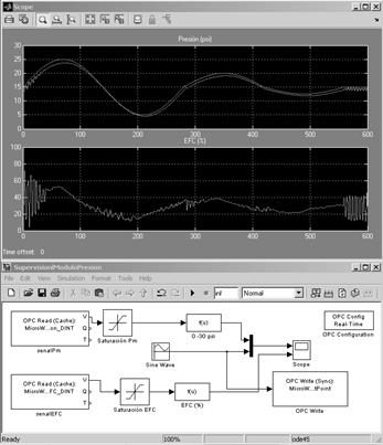
In order to visualize the process variables and the controller performance, it is recommended that an additional OPC-compatible application be created, which can be connected to the OPC server to acquire and plot the data of the desired process variables. In this work, a model was implemented in SIMULINK and was used as a client application for reading and visualizing the process variables from the OPC server. In order to work with this SIMULINK model, a license for the MATLAB OPC Toolbox is required. Figure 7 shows a simple SIMULINK model which allows us to connect with the OPC server and build the dynamic plots of the process variables we are interested in.
Implementation of the control system and start-up
Once the required files have been created, the control system can be implemented and started up by connecting the SIMATIC S7-200 PLC and the computer through a TCP/IP connection cable. The control system is started as follows:
1). Run the simulation of the SIMULINK supervision model.
2). Run the OPC connection with the EMSO model in the respective EMSO-OPC project.
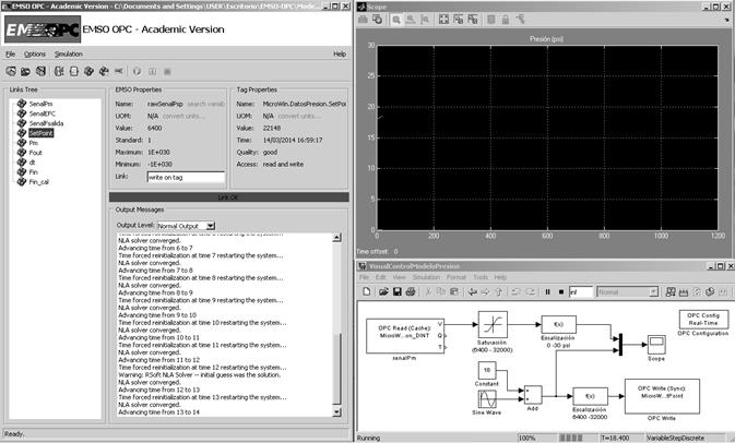
By using the methodology described in section 2, two control systems were stated: (1) a single-loop feedback control system with a PID controller and (2) a control system based on the process model obtained in section 4. The screenshot in Figure 8 shows how the control system based on EMSO and implemented via OPC (left-hand side) can be coupled with the supervision system in SIMULINK (right-hand side) in order to provide a simple control system connected in real-time to a process module.
Single-loop control system using a PID controller
In order to state this control system, a mathematical model had to be built to describe the PID controller. In the literature, there are a lot of models for describing PID controllers [13,14]. However, in this work we only used the ideal form of a PID controller described in [14], as shown in Equation (18).
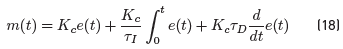
Where, m(t) is the output signal leaving the controller expressed as a percentage (%). Figure 9 shows the statement of the PID controller model in EMSO.
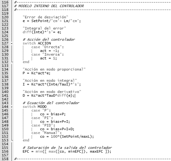
The performance of this controller for different disturbances in the Set-Point is discussed in subsection 3.4.
Single-loop control system based on the PBSM model
In order to state the control system based on the Phenomenological-Based Semiphysical Model (PBSM), the operating mode of the process module which we were interested to work with (described in section 3) had to be selected manually. In this subsection, a simple controller based on the PBSM is stated. This controller was used to govern the liquid level in tank TK-01 by regulating the liquid flow coming into the tank. The controller stated here is a short version of the complete PBSM stated originally and was designed to work with only one of the tanks, TK-01 in this case. This is because is one of the most widely used controllers in the process control laboratory. However, working in a similar way, it is possible to obtain specific controllers based on the PBSM for each of the rest of the operating modes.
If only TK-01 is considered, it is assumed that the liquid level never goes beyond the cylindrical section of the tank. When using the model Equations (1),(5),(6),(9),(11) described in section 3, a reduced form of the mathematical model can be obtained, as shown in Equation (19), which allows the manipulated variable to be computed directly.
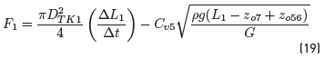
Where, 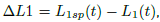 represents the deviation error in the controller,
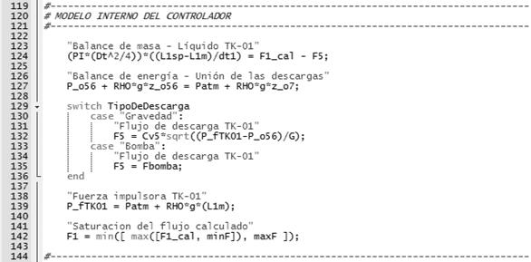
  corresponds to the sampling time used for the controller computations and the other terms corresponds to parameters of the model. Figure 10 shows the PBSM-based controller model as stated in EMSO.
In general, these controllers were implemented via OPC in the laboratory by scaling the input and output variables of the controller models from and to the range [6400, 32000] respectively because this represents the range of analog signals in the SIMATIC S7-200 PLC.
3.4 Analysis of controller performance
Figures 11 and 12 show the performance of the PID controller and PBSM-based controller for different disturbances in the Set-Point. In the case of the PID controller, the parameters used were 𝐾 𝐶 = 10.9307, 𝜏 𝐼 = 61.2497 𝑠, and 𝜏 𝐷 = 4.4192 𝑠. These parameters were obtained by process identification assuming a first-order-plus-dead-time dynamics (FOPDT) followed by the implementation of different tuning rules (Ziegler-Nichols in closed-loop [15], Tyreus-Luyben in closed-loop [15], Ziegler-Nichols in open-loop [14], Cohen-Coon in open-loop [16], Minimum integral error criteria of López et al. and Rovira et al. [14], and the Ciancone correlations [17]). Each controller obtained was tested in the real system. As result, the Tyreus-Luyben controller was selected due to the best performance.

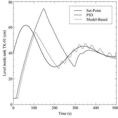
Although both control systems worked well for step disturbances of the Set-Point, it is clear that the PBSM-based controller was faster in reaching its final condition and it had a smaller overshoot than the PID controller. The PID reached the final value, but the PBSM-based model shown small continuous oscillations. With respect to the trajectory imposed for the Set-Point, it is clear that both controllers tried to reach the path. However, the PID controller failed severely compared to the PBSM-based controller. In general, the performance of the PBSM-based controller was good despite the small continuous oscillations observed in its responses, oscillations that could appear due to the time delays generated with the sampling time of the EMSO-OPC interface and the computation time used by the simulator.
4. Conclusions
In the present work, a basic methodology was proposed for controlling and supervising a process via OPC using the EMSO simulator and a SIMATIC S7-200 as an OPC communication interface. This methodology was illustrated by identifying and modeling a laboratory module process using the EMSO simulator. The model obtained was used directly in the design and implementation of a model-based control system via OPC. The PBSM stated for the process module was in very good agreement both qualitatively and quantitatively with the experimental data obtained, and it produced low deviation errors. Regarding the control systems implemented, in general the performance observed for the controllers was good. The PID controller worked well for step disturbances of the Set-Point, but it failed for an imposed Set-Point trajectory. On the other hand, the PBSM-based controller did a great job in both cases, despite some small and continuous oscillations around the Set-Point. In addition, time delays were observed when coupling the EMSO simulator, the EMSO-OPC interface and the real process module, due to problems in the synchronization due to the time delays generated by the sampling time of the EMSO-OPC interface and the computation time used by the simulator. As final note for future works, it was observed that varying the sampling time parameter can improve the performance of the control system.