


 Inglés (pdf)
 Articulo en XML
 Referencias del artículo
 Enviar articulo por email
 Citado por SciELO
  Citado por Google
  Similares en
SciELO
Similares en
SciELO  Similares en Google
 Permalink
1. Introduction
In system dynamics theory, it is common to study different types of systems representing a real model, such as biological, financial, or human behavior. Thanks to the different scientific sources of knowledge, it is possible to have a good understanding of the physical properties of the systems and their representation using differential equations.
However, complete information about the system is not always available. Typically, complex models (non-linear models) have unknown dynamical parameters and since they cannot be directly measured, they must be estimated. Parameter estimation has been a challenging process for different models, due to the following reasons: the large amount of parameters, the technique used for optimizing the objective function, and the selection of an accurate estimation methodology. Some research projects have addressed the estimation problem using methods that are theoretically not exact but give good approximations. These methods are the heuristic algorithms. Authors in the following works [1-4] used heuristics techniques for parameter estimation in dynamic systems when they were facing a non-convex objective function, or a very costly computational solution, due to the large amount of variables.
All the theory is supported by a careful study of the linear system representation. Nevertheless, the importance of tackling models with non-linear representations is well-known. Different phenomena in biology, engineering, etc. are represented with one of the multiple general linear models that have been proposed in literature. As far as the biotechnological branch is concerned, there are studies of different complex models represented by a dynamic system such as the work by [5].
In the current work, we focus on the complex model of the Zymomonas mobilis fermentation to produce etanol [6,7] with the objective of estimating its set of parameters.
The chosen use-case is a topic with a special role nowadays, since world energy consumption has been increasing during recent years due to mass production generated by the growing technologies in production processes and the consumption demands of a growing human population. The limited reserves of fossil fuels have increased awareness about the significance of finding substitutes for the traditional non-renewable energy source. Therefore, biotechnology has made significant advances aimed to fermentation technology of ethanol. An advantageous ethanol producer is the mentioned Zymomonas mobilis, since its yields are the highest reported in literature. This bacterium has an ethanol yield close to the stoichionetrical value of 0:51 g ethanol/g glucose [8]. Another benefit of using it for etanol production is its high tolerance to elevated temperatures enabling to reduce costs of cooling during fermentation and to increase productivity [9].
Unfortunately, Zymomonas mobilis exhibits a non-linear and oscillatory behavior, besides, some states and parameters of the fermentation process are not possible to measure. The unknown states are biomass concentration and the inhibition effect. It has been demonstrated that the inhibition effect against substrate is more due to ethanol concentration than to substrate concentration, thus, productivity of Zymomonas mobilis fermentation yields depends on the feeding strategy [9]. Therefore, in order to measure the rate of ethanol production, it is crucial to measure intermediate variables to describe the inhibition effect as well as other important parameters. Hence, in this work we are interested in demonstrating that, applying and improving different heuristic methods found in previous works, it is possible to estimate the set of parameters for the fermentation process as well as for other complex bioprocesses with a good performance. This would allow a better representation of the models of different bioprocesses which would contribute to the industrial area. So far, one of the best heuristic algorithms for this problem is the Particle Swarm as shown by [2].
In order to hit the target in this work, we may use the result of previous research projects to create an initial solution for all the algorithms. Previous works which have worked with the full non linear systems [5-7,10] were necessary for this aim. Furthermore, we implemented each algorithm in the Python computing language, and then we carried out a performance analysis by matching both the computational time and the value of the objective function. This work is organized as follows: the following section will describe briefly the nonlinear nature of the system under study and some elements that we are going to use. Further, section 3 summarizes the heuristic methods to be implemented. Section 4 is dedicated to analyze the results of the previous section and finally, section 5 contains our concluding remarks.
2. Non-Linear System Description
The non-linear space system is presented in great detail in [5,6,10].
When simulating the non-linear system, it is posible to observe the open loop behavior in each state. The initial conditions considered in this model for our research are the following:
Biomass: 1.5 g/L (first state) (X)
Substrate: 57 g/L (second state) (S)
Product: 57 g/L (third state) (P)
Ethanol: 0 g/L (fourth state) (W)
Inhibition effect: 0 g/L (fifth state) (Z)
It is known in the open loop behavior of Zymmomonas mobilis model that the biomass, substrate and product states keep the oscillatory behavior during the entire experiment. Real data also exhibits the same behavior based on the model presented by [2,6].
In equation 1, the state space representation of the Zymmomonas mobilis system is presented:
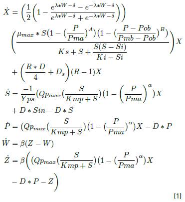
where D = Ds + Dr, Dr= 0 and R is the biomass recycle rate.
The real experimental results of the system of Zymomonas mobilis that we study are analyzed in the work of [6,9,10].
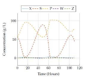
Figure 1 presents the real values for the 5 states (X, S, P, W, Z) during a 110 hour simulation of the Zymomonas mobilis system:
As we can see from figure 1, the two observed states (S and P) have very similar scales of magnitude and have a related behavior. We consider these states to be the most important states and therefore we focus on analyzing their behavior in this figure. During the simulation, they oscillate through certain periods of time and the relation between them seems to be inverse: when one of them increases the other seems to decrease and vice-versa. The other states present very small scales of magnitude when compared to S and P, yet we can still see an oscillatory behavior in stateX from this plot. The behavior of these real values of the states is shown better in the plots presented in the experimental results section.
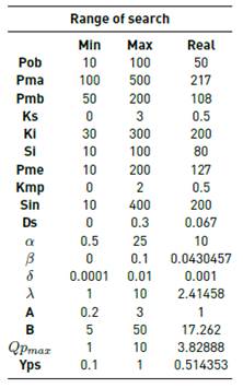
For each of the parameters that we needed to estimate, we defined arbitrarily a minimum and máximum posible values to limit the solution space, based on the scales of their values in the real model (it is clear that the real value of each parameter is therefore contained within this interval, that is between the minimum and máximum possible). It is important to mention that all of these parameters are continuous. Predefining these searching ranges for the parameters allows a fair comparison between the results obtained by the different heuristic methods, as seen in the literature [11].
The initial solution that we would use for many of the heuristic methods consisted in selecting the middle point of this interval (which is the same as the median between its maximum and minimum posible value). Table 1 presents the search ranges for each of the parameters of the model, along with the real value.
3. Heuristic Methods
As it was mentioned before, many heuristic techniques were implemented in order to determine which of them provide the best result for the parameter estimation in this model. The following section describes each of the heuristic methods that were implemented.
3.1 Iterated Local Search
A local search technique was proposed for this problem. The local search for a particular set of parameters consists of making small variations in just one of these parameters. These variations are either small increments or decrements in its value, while keeping the rest of the parameters constant. Then, we continue increasing or decreasing the value of this parameter in small rates until the solution does not improve anymore. Once this is achieved, we continue from the best found solution by further varying a second parameter, while keeping the first one and the rest of the parameters now constant. So we again change up and down the value of this second parameter by small steps, until the found solution does not improve any more in terms of the objective function. We repeat this process for all of the remained parameters, and even cycling it, by starting again varying the first parameter but in a completely different (and better) solution, until we find that the solution does not improve anymore no matter which parameter is varied (local optimum).
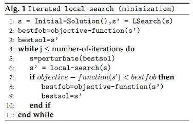
The local search method was used in a more efficient and general algorithm known as iterated local search [12]. In this method, an initial solution is chosen and local search is used to find the local optimum, but when this happens, the local optimum is perturbed to find a new solution. The perturbation in this case consists of varying each of the parameters of the local optimum in a certain percentage (either increasing or decreasing it; the percentage of variation is different for each of the parameters of the solution). After this, a completely new solution is obtained, and when we apply the local search technique to this solution it would probably find a completely different local optimum, which may be even better than the one previously found. We repeat this same process of perturbing again the best found solution and then applying local search many times. This process allows us to explore deeply the solution space to obtain even better solutions than with a simple local search method. Figure 2 presents the structure of the Iterated Local Search algorithm.
3.2 Genetic Algorithm
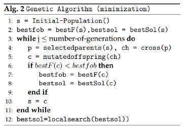
A genetic algorithm [13] is an heuristic method that belongs to those called population heuristics. In this kind of techniques, a population of solutions is used to produce and obtain new solutions that may provide a better objective function value for the problem. In a genetic algorithm, first an initial set of solutions is created, and this will represent the first generation of the algorithm. In this case, that first set of solutions is constructed in a completely random way. The next step is evaluating the objective function for each of these solutions (the best one of them is stored), and then using a selection criteria to choose which are the solutions (“parents”) that will be used to create new solutions (“offspring”). Usually, good solutions are selected more frequently than bad solutions.
For this algorithm, the selection criteria is the roulette, in which a probability of being chosen is assigned to each solution, where better solutions have higher probabilities of being selected. The next step is using the parents population to create new solutions: this is done by using a crossover method, which combines characteristics of the parent solutions to produce new solutions. For this case, an uniform crossover was selected, where the value of each parameter of the solution is given randomly by one of two parents used with a 50/50 chance. After all the offspring has been generated, some of them (in this case 5%) are mutated, to be able to explore even more the solution space. The objective function value is calculated for all of them, and the solution with best objective function is saved if it is better than the one found before. The population of offspring then becomes the parent population for the next generation, and the process is repeated for many generations, which allows a deep exploration of the space of solutions to search for a very good solution in terms of the objective function. This algorithm at the end of its generations includes a local search method to improve the objective function in a local area. Figure 3 presents the structure of the Genetic algorithm.
3.3 Variable Neighborhood Descent
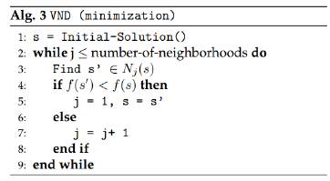
The variable neighborhood descent algorithm [14] is found on the set of local search algorithms: it starts with an initial solution and creates a neighborhood for it. Then, among all possible solutions contained in the neighborhood, it finds the first solution that has a better objective function value than the initial one, and this one is saved as the best solution. Then, for the new current best solution, a new neighborhood is generated and the previous process is followed iteratively until the stop criteria is reached.
This method, as well as the other methods based on local search, has a good performance when trying to find an optimal solution for a problem, since its convergence time is not too high. Furthermore, depending on the initial solution that is given to this algorithm, it is possible to reach different local optima in which the solution would no longer improve anymore. Moreover, this method is easy to implement because of its structure. Figure 4 presents the structure of the Variable Neighborhood Descent Algorithm.
3.4 Random Search
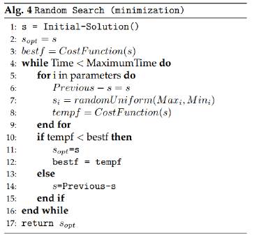
Random search algorithms have proved to be efficient for parameter estimation problems in the literatura [15]. This version of the random search algorithm is not as random as the name implies: the algorithm does a kind of local search but with a random factor. It starts from an initial solution and within each iteration it modifies only one of the parameters of the solution. If this alteration improves the objective function, then the best solution is updated. Then it goes further by modifying the next component of the solution in the next iteration, and it repeats the process for all the components of the solution.
The random side of this algorithm is related to the solution modification: when the parameter of the solution is changed, it will take a random value between the search range of values for that component or parameter. Figure 5 presents the structure of the random search algorithm.
3.5 Simulated Annealing
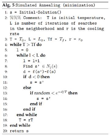
The simulated annealing algorithm was used the first time on combinatorial optimization by [16]. This algorithm is one of the first methods with a probabilistic acceptance criteria: a solution is replaced with an specific probability.
Some of the parameters of this technique are the value of temperature (T), the ratio the temperatura decreases (r), final temperature (Tf) and the number of solutions to look for on the neighborhood. In the current work, we proposed as empirical values T = 100, Tf = 0.1, L = 200, r = 0.7.
The advantage of this algorithm, is that it uses the techniques of a local search method (trying to improve its solution in each iteration looking for a feasible solution in a neighborhood) but instead of analyzing the performance of each solution, it calculates the likelihood of acceptance of each solution. This criterion does not allow the method to consider bad solutions in its search range.
Furthermore, after each iteration the acceptance criterion becomes more exigent when calculating the likelihood to accept one solution that can be considered as a good solution. Figure 6 presents the structure of the Simulated Annealing algorithm.
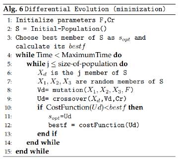
3.6 Differential Evolution
The differential evolution version that has been implemented was taken from [17]. According to this method we must consider the following parameters: F =mutation ratio, F ϵ (0; 2), Cr =crossover ratio, Cr ϵ (0; 1), kmax =number of search iterations or maximum execution time.
In this algorithm, the first step is to initialize the population S: a random initial population is generated, conformed by p = 40 individuals. Then, in the second step, it evaluates the fitness function or cost function for all the individuals in the population in order to find the best solution and sabe it as s opt , it also saves its fitness value as best f.
In the third step, an individual test X d is chosen and other three individuals are randomly selected from the population: (X 1, X 2 and X 3), in such a way that they are different among them and also different from the individual X d . In the next step, a mutation is calculated for the individuals already selected: V d = X 1+F*(X 2 - X 3). After this, it comes the crossover operation between X d and V d in order to obtain U d .
Finally, the algorithm evaluates the fitness function or cost function again, this time for U d (the resulting individual from mutation and crossover operation), and it compares its cost function value with s opt fitness value. If U d fitness value is better than the one of s opt , then s opt = U d is made. However, if the cost function does not improve, the best known solution s opt remains the same. A new individual test X d is chosen and the process is then repeated through many iterations until the maximum number of search iterations of kmax is reached.
If the reader is interested in understanding the exact process and formulas used to perform the mutation and crossover operations, he can use as a reference the work presented in [17]. Figure 7 presents the structure of the differential evolution algorithm.
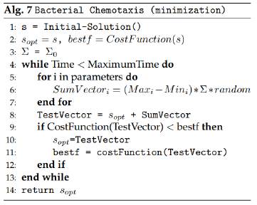
Bacterial Chemotaxis
The bacterial chemotaxis algorithm [18-20] makes a random walk and moves towards the gradient of sugar concentration. It also has a Σ parameter which weighs the movement amplitude. This heuristic technique is applied by executing the following steps:
1. Generate an initial solution as a vector of initial parameters. (At the start, this initial solution is labeled as the best found solution). The current best objective function (the objective function of this initial solution) is also calculated and stored.
2. Create a summation vector which will then be added to the current best solution (initially this one is the initial solution). The summation vector is created by considering the maximum and mínimum values for each parameter, and it will represent a positive or negative value for each of the parameters that will be added to the best known solution (this summation value is calculated randomly for each of the parameters). This summation vector is the one that allows us to produce a random walk when adding it to the best found solution and therefore explores the solution space.
The summation vector is generated with the following formula: for each parameter i of the best known solution, we generate a random number from a certain probability distribution (this is one of the execution parameters of the algorithm). This value can be either positive or negative. Then, we multiply this randomly generated number by the amplitude of the interval of possible values for parameter i (the amplitude is the difference between the máximum and minimum values of i). Finally, we multiply the obtained result by a factor Σ which determines how big are the steps that we may use in each iteration (the selection of the parameter Σ is also an execution parameter).
Therefore, each value of the summation vector is the result of multiplying a random number by the amplitude of the interval of each parameter and then multiplying this result by the Σ factor.
The next formula shows its estimation:
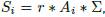 where Si is the value for position in i of the summation vector, r is a randomly generated number, Ai stands for the amplitude of the parameter that is estimated in the position i of the vector and Σ is the multiplying factor.
For example: if we have a parameter i whose posible values vary between 1 and 3 (that is, with an amplitude of 2), and we use a uniform distribution between -0.1 and 0.1 and a Σ factor of 0.05, in order to calculate the value of the summation vector for this parameter we apply the formula as follows:

It is important to note that, in the calculation of the summation vector for each parameter, the probability distribution used and the Σ factor are the same, but the randomly generated number and the amplitude of the interval vary, thus we obtain a different summation value for each parameter.
3. A new solution is calculated by adding the parameters of the best known solution and the parameters of the current summation vector. This new solution is called the testing solution. We compute the objective function value for this testing solution.
4. If the value of the objective function for the testing solution is better than the one of the best known answer, we change the parameters of the best known vector with the parameters from the testing solution. Otherwise, we just discard the testing solution.
5. The iteration from steps 2 through 4 is performed many times, thus creating each time new testing solutions and comparing them against the best known vector of parameters. This process is repeated for a certain amount of time in order to explore the solution space and evaluate many different solutions, allowing us to obtain a very good answer with this method.
Figure 8 presents the structure of the Bacterial Chemotaxis algorithm.
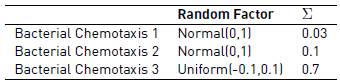
In this study, we consider three different versions of the bacterial chemotaxis algorithm, in which we vary both the distribution of the random factor and the value of the Σ component. Table 2 shows the characteristics for each version of the bacterial chemotaxis algorithm.
4. Experiments Results and Analysis
In this section we present the performance and analysis of the heuristics introduced previously. All the heuristics were designed to optimize the value of a common objective function, which measures the distance between the estimated states and the real states, taken from the work [5]. Therefore, the smaller the objective function, the closer we are to estimating correctly the system of Zymomonas mobilis. Hence, we evaluated the performance of the algorithms in terms of the objective function.
To test the performance of the heuristic methods, two computers were used. For the 3 hours run, we used a computer with Windows 10 64 bits, 8 GB RAM, Intel core i5 processor and 2.2 GHz. For the 5 minutes run, we used a computer with Windows 10 64 bits, 4 GB RAM, Intel core i5 processor and 1.8 GHz.
4.1 Analysis of the results in terms of objective function
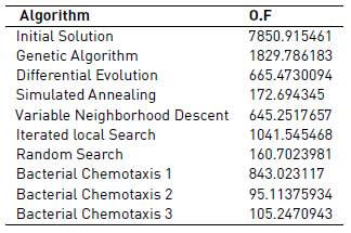
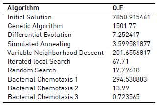
The objective function selected was the mean squared error (MSE). In Tables 3 and 4, it can be seen the results from each algorithm regarding the objective function.
4.2 Experimental Results From the Model for Each Set of Estimated Parameters
Here, we present the results obtained by simulating the model for a time of 110 hours with the parameters estimated by each algorithm. These parameters were estimated in two scenarios: after 5 (five) minutes and 3 (three) hours of execution.
We show results for the four selected algorithms which had the best performance (based on Tables 3 and 4] in terms of the objective function: Simulated Annealing, Differential Evolution, Random Search and the best versión of bacterial chemotaxis, version 3. The performance of each of the algorithms is also showed in a more visual way: presenting the real behavior for each state of the model in Figures 9 to 18.
Other heuristic methods (genetic algorithm, variable neighborhood descent, iterated local search and the other version of bacterial chemotaxis) did not give as good results as those obtained by the four algorithms mentioned before. Thus, their results are not plotted. Analysis for the model response with different sets of parameters estimated is also carried out.
We have multiple versions of the chemotaxis algorithm: for the 5 minutes execution, versions 2 and 3 are the ones that provide results that are closer to the real model, specially for substrate and product. Version 1 does not provide very good results in comparison to the other 2 versions. Versions 2 and 3 provide decent results for such a short time.
Then, looking at local search algorithms, they give a decent performance in terms of objective function. There were not as good results as those obtained by the bacterial chemotaxis. For the 5 minutes execution, variable neighborhood descent and random search algorithms performed similarly, being able to obtain more or less acceptable solutions but not as good as with the bacterial chemotaxis algorithm.
Random search proves to be the best algorithm among the three local search based methods after 5 minutes of execution. Meanwhile, Iterated local search is the method which gives a lower performance in comparison to those obtained with the other two methods based on local search. In addition, after 3 hours of execution, we noticed a change in comparison to the 5 minutes execution: now the iterated local search algorithm provided almost as good result as the random search, while the variable neighborhood descent did not perform well.
Furthermore, results obtained for 5 minutes execution using the genetic algorithm were bad, while the simulated annealing and differential evolution algorithms provided acceptable results, but again not as good as the ones obtained by bacterial chemotaxis. The same behavior was observed after increasing the execution time up to 3 hours.
Figures 9 to 18 show the results for the states obtained by the simulation with the parameters estimated by the selected four algorithms. For the simulation, we labeled for each time step (hour) the value of each state (concentration, measured in g/L).
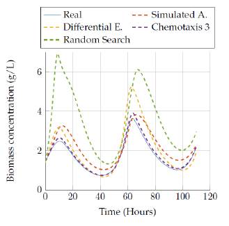
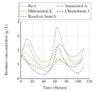
Figures 9 and 10 show the comparison of the results obtained by the best four heuristic methods in the biomass state. It is possible to see that simulated annealing and version 3 of bacterial chemotaxis provide good results for the 3 hours run. Also, a pattern in this state regarding the behavior of the estimated values is observed, since a lower run time gave us solutions below the real data, but increasing the run time gave us behaviors above the real data.
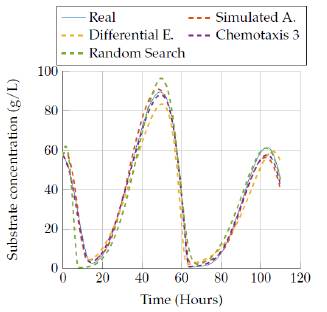
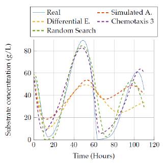
Then, figures 11 to 12 show the comparison of the results obtained by the four algorithms in the substrate concentration state, where it can be seen that the random search algorithm and the last version of the chemotaxis algorithm provided a really good approach whereas Simulated annealing and differential evolution lost accuracy when trying to represent this state with a low execution time. Moreover, a really good estimation was obtained after 3 hours of execution, since those algorithms fit very well the model behavior as it is seen in figure 10.
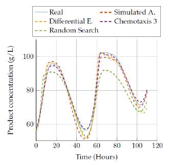
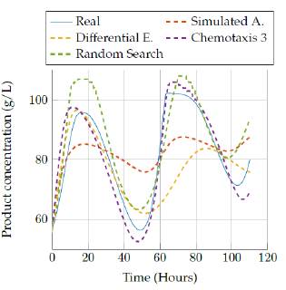
Figures 13 to 14 allow comparing the results obtained by the four algorithms in the product concentration state. The outputs for this state have a similar behavior to the previous state, where the random search algorithm and the last version of the chemotaxis algorithm provided a really good approach independent of the execution time. But again, the Simulated annealing and differential evolution lost accuracy when the execution time was very low.
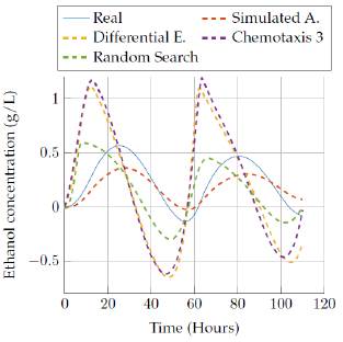
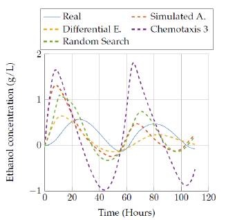
In figures 15 to 16 the results obtained by the four algorithms in the ethanol concentration state are also compared. It can be seen the big difference of the estimated state against the real, since none of the estimations gave a really good representation with the execution time. However, the random search algorithm and Simulated annealing algorithm provided a representation that was close to the real values after 3 hours of execution.
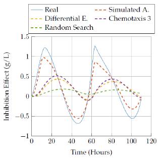
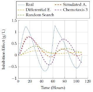
Figures 17 to 18 compare the results obtained by the four algorithms in the inhibition effect state. Once again, it was not possible to get a more accurate representation for the state with low time execution for the algorithms, but increasing the time up to 3 hours allowed the Simulated Annealing algorithm to get a closer representation of the real behavior.
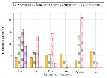
Another way to analyze the algorithms performance is calculating their estimation error. For this aim, we took into account the real value of the parameters [Table 1] and calculated the relative percent error for the list of parameters. In this task, we noticed that the estimation skills of the heuristics vary depending on the parameter, which might be due to the different ranges of the parameters. In figure 19 we showed the percentual estimation error of six of our parameters in order to see the general performance of the algorithms in this model. As it can be seen, the chemotaxis 3 was the algorithm with the lowest estimation error in this group of parameters; it was even the heuristic with the closest estimations to the real values in the simulation of the states. However, for some parameters, the chemotaxis 3 did not have the best estimation, as it can be seen for the parameter “Pob”. Differential evolution had the lowest error for estimating the “Pob” parameter. In general, the heuristic estimation errors are under the 50%, which is acceptable considering the good results of the simulations with the parameters estimated.
4.3 Analysis of the Results of the Model with Parameters Estimated with each algorithm
One of the important things to analyze is that although many of the estimated parameters were able to obtain good results for the states S and P, the same sets of parameters many times did not provide good results for the other three states X, W and Z. This happens because the selected objective function was the mean squared error and the scales of the variables were very different (P ans S had values near 50, while the remaining three variables had values that were very low (usually lower than 1 for W and Z and lower than 1 for X). Therefore, when trying to minimize the cost function, the algorithms always gave way more importance to minimizing the errors of P and S, even if it meant generating bigger errors in the other three states. This may be explained due to the big difference in scales: an error of the same percentage in variables S and P would lead to a much higher cost value than an error in the same percentage for the other three variables. While trying to minimize the error, the algorithms prioritized the correct estimation of S and P. Although this could have been avoided by normalizing all of the state variables, this was not done because in the literature for this model the two outputs are almost always P and S, and therefore we considered that the algorithms should prioritize estimating these two states in the best possible way.
Now, it is time to focus on the accuracy of each of the algorithms:
As far as the genetic algorithm is concerned, it takes a random population of possible solutions (including the initial solution) and the crossover process is done without a good criterion (each parameter is given randomly either by the mother or the father, but they do not cross to créate new non existing parameters). This creates solutions that do not fit to the real system.
Differential Evolution is an algorithm similar to the genetic. It performs the process with a high computational cost, as mutation and crossover. So, for short time runs, as 5 minutes, the algorithm is not very accurate, but when the period of run increases, it has time to perform many iterations, so it can go over almost the whole solution space and therefore, the solution improves considerably.
Although the Iterated local search algorithm is able to provide good solutions, a high computational cost is required by it, because it has to consider all posible parameters variations in each iteration. In general, local search algorithms tend to consume high computational resources since they have to explore the local area for each of the parameters of the solution.
Variable Neighborhood Descent algorithm (VND) can provide good solutions, but just as in the local search algorithm, a high computational cost is required. This is because this method consists in finding neighbors of the solution using random values for each parameter, which leads to a higher computational time required. By using this technique, it is possible to explore broadly the solution space, but without a good criteria for determining the neighborhood, the convergence of the algorithm is very slow.
Random search as it was explained above, is not as random as its name implies, it does make an intelligent solution search. The reason why its results overcome the Iterated Local search and the VND, is because this method has a low computational cost: it is very easy for the machine to generate neighbors of the solution on each iteration, since it only has to modify one parameter of the solution each time (this modification is random). As we could see on the results for 5 minutes and three hours, the accuracy improves as time increases. Since this method is very susceptible to generate very bad neighbors, due to its random factor, so for a short run, say 5 minutes, the algorithm does not have enough time to generate many neighbors and the initial solution Will not improve subsequently. However, when the algorithm runs for longer periods it has time to make a considerably amount of iterations that allow improving the solution considerably, overcoming other methods that may generate better neighbors but with higher computational cost.
Simulated annealing algorithm is a searching method similar to the common local search, but this algorithm has an acceptance criteria in each iteration for a posible solution. This criteria allows the algorithm to look for good solutions in the space of solutions quickly and therefore it has a good performance for short and long times of execution.
Bacterial chemotaxis algorithm is a method based on a simple technique (disturbing each parameter of the solution in each iteration), and with this methodology we can explore the space of solutions. This technique has a very good performance for both long and short times (this heuristic allows us to evaluate many different solutions very quickly, therefore allowing us to find very good solutions in a short time).
When comparing the three different versions of the bacterial chemotaxis algorithm, we noticed that choosing a correct value for Σ is a key factor in the algorithm efficiency. We found out that for short execution times (5 minutes) a medium value of Σ provided the best results. This is because for such a short time just a few solutions can be evaluated, and a value of 0.1 provides the correct equilibrium between exploration (search in the global space) and exploitation (search in the local space). Different results are seen in the 3 hour time lapse: in this case, there is a lot of time to exhaustively search the solution space, and therefore in this case we should use a higher value of Σ of 0.7 to obtain the best results (this value of 0.7 allows us to search a wider area of the space of solutions).
To summarize, we have seen that population heuristics can provide acceptable results only if the crossover combined parameters from both parents, like in Differential Evolution (genetic algorithm did not provide good results). However, differential evolution converges slowly and provided very good results in 3 hours execution, but in 5 minutes execution its results were not that good.
On the other hand, all of the local search algorithms required a very high computational time to be able to obtain pretty good results, and therefore did not perform very well in the 5 minutes execution. However, in the 3 hours execution, results for Simulated Annealing, Random Search and Iterated Local Search algorithms were very good (variable neighborhood descent did not have good results).
Therefore, the algorithms that provided a better performance regarding their objective function, their efficiency and how well they fit the real system, were the bacterial chemotaxis algorithms. This is because of the criteria that these algorithms must follow, when looking for solutions: their criteria allow them to explore quickly a large number of solutions, and thus they can improve the quality of the best found solution very frequently. Bacterial chemotaxis has a great advantage against all other algorithms in the short execution time of 5 minutes, and a slight advantage over other techniques like local search based and differential evolution in the 3 hours execution (we should also note that in this 3 hours execution, results obtained with the parameters estimated by version 3 of the bacterial chemotaxis were very good and almost identical to the real model).
5. Conclusions
For bacterial chemotaxis it is better to choose a big value for Σ when the run time is long, but it is better to choose a medium value when the run time is shorter. This is because Σ determines the size of the steps, and when the time is longer we are more capable of exploring larger areas in the solution space. Therefore the steps made by the solution vector can be greater.
Heuristic techniques based on local search are good algorithms for estimating parameters for this model in long running times, but not equally good for shorter periods of time. This is because performing a local search has a high computational cost and in short periods of time these techniques are not able to explore many different solutions. However, performing local search is a good way to improve the solution quality in a local area in larger periods of time. Simulated annealing is also based on searching the solution space and it also required long periods of time to obtain very good results.
Differential evolution is much better than the genetic algorithm since it combines the parent parameters to create new parents, while the genetic algorithm only chooses each parameter randomly from one of the parents (does not create new parameters in the crossover).
Among all the designed and compared algorithms, bacterial chemotaxis proved to be the best for both short and long periods of time: in the 5 minutes execution, versions 2 and 3 had very decent results and were able to represent the real model way better than any of the other algorithms, while in the 3 hours execution, version 3 of this algorithm was the best of all and was able to obtain results that were almost identical to those represented by the real model.
A careful selection of the best heuristic technique for a particular parameter estimation problem proved to be very important to be able to obtain the best values for the parameters to simulate the behavior of the system.
Some of the tested heuristic techniques were able to provide very good estimations for the Zymomonas mobilis model, which is a very complex non-Gaussian system. Therefore, estimating the parameters for the model by using heuristic methods seems to be a good approach for solving this problem.

