


 Inglés (pdf)
 Articulo en XML
 Referencias del artículo
 Enviar articulo por email
 Citado por SciELO
  Citado por Google
  Similares en
SciELO
Similares en
SciELO  Similares en Google
 Permalink
1. Introduction
International standard ISO 9613 Part 2 specifies an engineering method to calculate sound attenuation during outdoor propagation and to predict sound pressure levels at a certain distance from various sources [1]. In this method, the source of noise emission is considered as a point source and sound emission at any receiver is predicted with reasonable accuracy under conditions that are favorable for the propagation of sound [2].
However, in 2006, van den Berg demonstrated that this calculation results in significant underestimations of the expected sound levels at the receptor; moreover, these levels occur primarily in atmospherically stable conditions. Furthermore, with the increasing height of wind turbines, the difference between the real and estimated sound pressure levels increase considerably [3].
Unfortunately, the problem of noise propagation from wind farms is not easily solved. Significant fluctuations in sound pressure levels obtained from areas surrounding wind farms that are currently in operation are revealed. A large part if this variation may be attributed to the fact that the power of the sound emitted from the wind turbine is a function of wind velocity; however, it is also known that the fluctuations are a result of changes in the sound propagation trajectory from the wind turbine to the receptor [4].
The uncertainty in predicting sound pressure levels using current analytical or empirical models may be significant and result in the failure to use valuable wind resources in order to avoid possible conflicts arising from the produced noise. If the sound pressure levels associated with wind farms are precisely calculated, the environmental acceptability of the proposed projects can be evaluated adequately during the planning stage [4].
2. Prediction of noise generated by wind turbines
The sound emitted by wind turbines is irradiated above the ground, usually at an altitude between 50 and 150 m. As the sound propagates, it frequently diminishes if the wind turbine is far from the receptor. The type of terrain and meteorological conditions influence the attenuation of the sound over distance [5]. The most commonly tools used to predict the sound pressure levels associated with fixed sources generally follow the calculation method proposed in the standard ISO 9613 Part 2.
The method established in standard ISO 9613 Part 2 is a general model to predict sound pressure levels at a specific receptor, which originates from known sources. It is a general method that can be applied to a wide range of noise sources and includes most of the main attenuation mechanisms. The method predicts the sound pressure level with an A-weighting filter with a long-term average using octave bands. The model assumes a downwind position and a moderate positive temperature with winds from 1 to 5 m/s, measured from a height between 3 and 11 m [1].
Given the wide range of uses for the noise prediction model in addition to the great variety of factors which influence sound pressure levels in an open field, no procedure exists to define a detailed model which would be adequate to estimate the sound generated by wind turbines [6].
According to Wondollek, wind turbines are not omnidirectional point sources, as proposed by the model from ISO 9613 Part 2 [7]; i.e., the sound pressure level varies according to the position of the receptor as a result of the directionality of the sound. According to Friman and Hoogzaad [8,9], the directionality of the sound is a function not only of the position of the receptor but also from the wind speed.
Wondollek and Kalinski et al. indicate that a wind turbine is more than a simple point source and presupposing a spherical propagation is contradictory and results in an underestimation of sound pressure levels at the receptor, particularly at larger distances [7,10]. A drawback of the model from ISO 9613 Part 2 is that it only has been validated for source and receptor heights of up to 30 m and distances of up to 1000 m with a precision of 3 dB [7,10]. It does not consider source heights greater than 30 m and does not take into account atmospheric variations over significant distances [10].
As stated by Wondollek, according to the ground attenuation equations of the model from the standard ISO 9613 Part 2, if the source is located at a height of 80 m (axis height) and the receptor is placed at a height of 1.6 m at a distance of 500 m from the source, the ground attenuation should be constant and equal to −3 dB (63-8000 Hz) for hard soil and 4.3 dB for porous soil (500 Hz). Above 125 Hz, soil attenuation should be approximately 0 dB for porous soil. Accordingly, porous soil would produce a ground attenuation equal to zero, whereas hard soil would result in amplification. Another fact that must be taken into account is that the source height has no influence on the ground effect when it is greater than 10 m, and the ground effect is independent from the size of the average area [7].
According to Wondollek, if the axis height is 80 m and the projected distance is less than 2,445 m, the ground attenuation would be zero for porous soil and 3 dB for hard soil. Therefore, it is implicit that the average size of the area plays no role in the ground attenuation in the model from the standard ISO 9613 Part 2. In contrast, at heights in excess of 10 m, the height of the source has no influence on the ground attenuation, another result which sounds unrealistic. These are other examples of how the model from the standard ISO 9613 Part 2 cannot be applied at considerable distances or when the source and the receptor are either very tall or placed at a considerable height [7].
3. Methodology
In this study, an experimental program is designed to test the accuracy of the prediction method developed by the standard ISO 9613 Part 2. This includes measuring the sound pressure levels under given weather conditions at various distances from a noise emission source and comparing them against the estimated sound pressure levels estimated by the standard ISO 9613 Parte 2.
The measurements were conducted in a wind farm belonging to Kentilux S.A. company, located in the department of San José (Uruguay), kilometer 41 national route number 1, near Paraje de Punta del Tigre. More precisely, it is located within a property belonging to La Magdalena farm. The wind generation park constitutes an installation of 20 MW of total installed power. It is integrated by 10 Vestas wind turbines with a rated power of 2.0 MW each, with an axle height of 80 meters. They are of the tripala type, with pitch control, with asynchronous generator of double feeding.
Different measurement sites were selected, all of which were downwind from the wind turbines, in an effort to achieve the best alignment with the wind turbines. The noise originating from the wind turbines was recorded and measured (sound emission or sound pressure levels) using a microphone placed at a height of 1.2 m from the ground at various distances downwind from the wind turbine (from 100 to 900 m). The primary control of the distances of the measurement points were carried out through the appreciation of the noise produced by other wind turbines; the nearest wind turbine must be the dominant source; otherwise, the measurement would not perform.
177 measurements were made in which the sound pressure levels, the meteorological variables and the distances between the source and the receiver were measured simultaneously. The sound was recorded continuously for at least 10 min, since, in the measurement of the wind speed for synoptic purposes, the average of 10 minutes is used to smooth the fluctuations of small scale, so that the wind report represents the synoptic scale. The meteorological variables were taken from a meteorological station located inside the wind farm that has sensors located at 40 and 80 meters high.
The safest way to take into account background noise is to ignore any measurement in which the sound pressure level is not at least 6 dB higher than the background level. Thus, assuming that background sound pressure levels have no influence on the measured levels, it leads to an error of less than 1 dB. This criterion was used here.
The adjustment of the prediction model to the experimental data led to the improvement and perfection of the model, which was then used to predict sound pressure levels at a specific receptor a certain distance from the wind farm for a wide range of weather conditions. The prediction model chosen as the basis for this study was the one proposed in the standard ISO 9613 because it covers the principal sound pressure attenuation mechanisms, although they may also be improved.
A detailed statistical analysis was performed using the data obtained in the field to study the dependence of the residual sound pressure level on the remaining parameters that were observed (independent variables) during the measurements.
The statistics software Statgraphics Centurion XVI version 16.1.11 was used to analyze the data and obtain the mathematical model. The variables that were inserted into the mathematical model were selected by the XLSTAT 2009.1.02 statistical software using of a Principal Component Analysis. The variables that exhibited a correlation with the residual sound pressure level (positive or negative and greatest to least) were introduced one by one into the mathematical model until an equation was obtained, which explained the difference between the measured sound pressure levels and their estimated values.
Using the data obtained from the measurements and comparing them with the estimated levels, a calculation procedure was developed to predict the noise emanating from a noise source. The calculation method includes the parameters that have been shown to influence the sound pressure levels.
The adjusted model shows the dependence or relationship that exists between the attenuation due to atmospheric stability and the remaining independent variables.
In order to determine how to simplify the model, the highest p-value is taken into account for the independent variables. If the p-value is lower than 0.05, it can be noted that a statistically significant relationship exists between the variables and a 95.0% confidence level. Therefore, no variable should be removed from the model. The R2 statistic indicates the percentage at which the model explains the variability of the dependent variable. The standard error of the estimation may be used to construct prediction limits for new observations.
This analysis presents the equation of the adjusted model for attenuation due to the effects of atmospheric stability. The data was processed to determine the correlation among the residual sound pressure level, wind speed, atmospheric stability, distance, and incidence angle.
For this purpose, a multiple regression was conducted to analyze the correlation between the measured data in which the dependent variable is the residual sound pressure level given by the method established by the standard ISO 9613 Part 2, with the following adjustments:
Directivity factor: The directivity factor takes into account the direction in which most of the noise irradiates from a source. The equations proposed by Brooks, Pope, and Marcolini agree with those expressed by Friman and Hoogzaad wherein the directionality of the sound depends not only on the position of the receptor with reference to the source but also on wind velocity [8,9,11-13].
For high frequencies, the sound directivity factor may be calculated using Equation. (1) [11,13,14]:
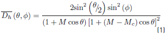
where  is the number of Mach from the supporting surface in motion,
  (
( ) is the number of convective Mach based on the flow at the trailing edge, and
  and
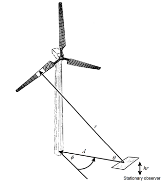
and  are angles of directionality, as shown in Figure 1. In this case, the angles of directionality are related to the wind turbine as a source of noise and its position with respect to the receiver.
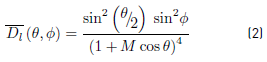
The directionality factor for low frequencies may be calculated using Equation. (2) [11,15]:
Attenuation due to geometric spreading: Martín Bravo et al. discovered that the propagation of sound from wind turbines resembles much more closely to that of a linear source model compared with a point source model when other factors are not taken into account [17].
According to the measurements made, the propagation model that exhibits the best fit for attenuation of noise from wind turbines over distance is that of cylindrical propagation, thus agreeing with the findings reported by Martín et al. It is precisely this model that presents the lowest residual sound pressure level.
The variation in sound energy as a function of distance using the cylindrical propagation model may be calculated using Equation. (3):
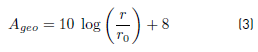
where r is the distance from the source to the receiver, in meters and 𝑟 0 is the reference distance (1 m).
Attenuation due to ground effects: The propagation of sound near the ground depends on the impedance level of the surface [18]. Porous surfaces allow sound to penetrate and therefore to be absorbed, submitting it to a change of phase through friction and thermal exchange [19].
Ground attenuation is calculated using the spherical reflection coefficient of the sound wave using Equation. (4) [20]:

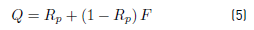
The spherical reflection coefficient is related to the reflection coefficient of the plane wave  by means of the Equation. (5) [20]:
Where  is the coefficient of loss at the limit of the interaction between the front of the wave and the finite impedance surface, which is a function of distance, ground impedance, and angle of incidence.
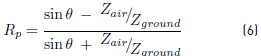
When the angle of incidence is greater than 5º, then → 0, indicating that the orb shape of the front of the wave needs not be taken into account [20]. The plane wave reflection coefficient is determined from the Equation. (6) [20]:
where:
 = Angle of incidence of the sound wave, °
 = Characteristic impedance of air at 20°C (415 Ns/m3)
 = Complex impedance of the ground, Ns/m3
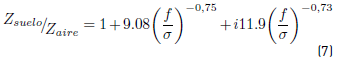
Various approximations have been formulated to determine ground impedance [20]. The Delany-Bazley model is characterized by its simplicity since it requires only one parameter, i.e., flow resistivity. It is an empirical model based on a regression analysis of acoustic properties and resistivity of airflow at the ground surface, which is represented by the Equation. (7) [21].
where:
 = Frequency, Hz
 = Resistivity of air flow at the ground surface, g/(s∙cm2)
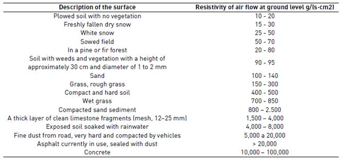
Typical values for airflow resistivity at the ground surface for different types of surfaces are shown in Table 1.
Attenuation due to effects of atmospheric stability. Atmosphere stability significantly affects the vertical wind profile and atmospheric turbulence [3]. Variation in temperature influences the density of air and consequently the velocity of the sound wave propagation.
The Equation. (8) presents the model proposed for attenuation due to effects of atmosphere stability:
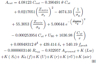
where:
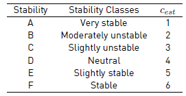
 = Class of atmospheric stability
 = Wind turbine axis height, m
 = Vertical propagation coefficient, m
 = Horizontal propagation coefficient, m
 = Angle of incidence of the sound wave, °
 = Parameter as a function of sound power levels, dB(Z)
 = Parameter as a function of the Strouhal number, dB(Z)
 = Parameter as a function of frequency, dB(Z)
 = Parameter as a function of wind velocity, dB(Z)
 = Parameter as a function of distance, dB(Z)
 = Parameter as a function of wind distance and velocity, dB(Z)
 = Parameter as a function of air properties, dB(Z)
 = Integral parameter of the boundary layer (equation 15), m
 = Peak frequency (equation 23), Hz
 = Reynolds number at a height of 10 m
 = Ground attenuation, dB(Z)
Table 2 presents the atmospheric stability classes and their relationship to the stability classes of Pasquill.
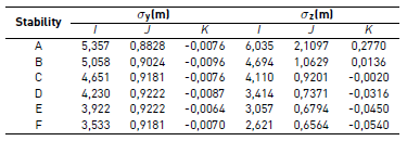
To calculate the horizontal and vertical propagation coefficients using a mathematical model, the Equation. (9) proposed by McMullen can be used [23]:
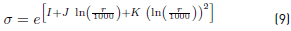
Where:
= Propagation coefficient, m
 = Distance between the wind turbine and the receptor, m
 ,
,  ,
,  = Empirical constants for each stability class
By comparing the dispersion of atmospheric contaminants and their relation to atmospheric stability, the horizontal and vertical dispersion coefficients from the Gaussian dispersion model were introduced into the multiple regression, resulting in a positive correlation between the coefficients and the residual sound pressure level established in the standard ISO 9613 Part 2. From this point forward, this article will refer to the dispersion coefficients as propagation coefficients.
The propagation coefficients represent the degree of vertical and horizontal dispersion of the sound pressure levels. High standard deviation values are obtained from an atmosphere that is unstable and turbulent, whereas low values are produced by less turbulent atmospheric conditions. Table 3 shows the value of the constants for McMullen’s equation.
The parameter of the sound power levels is given by the Equation. (10):
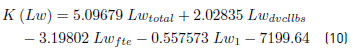
where:
 = Total sound power level, dB(Z)
 = Sound power level due to incident turbulent flow, dB(Z)
 = Sound power level due to detachment of the vortices of the laminar boundary layer at the trailing edge, dB(Z)
 = Sound power level in function of the wind velocity and the frequency, dB(Z)
The total sound power level in octave bands is obtained by integrating the contributions of all the acoustic sources through the Equation. (11):
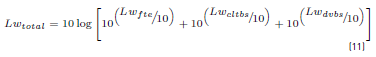
where:
= Sound power level due to incident turbulent flow, dB(Z)
 = Sound power level due to detachment of the turbulent boundary layer at the trailing edge, dB(Z)
 = Sound power level due to detachment of the vortices of the laminar boundary layer at the trailing edge, dB(Z)
The noise induced by incident turbulence is obtained by the Equation. (12):
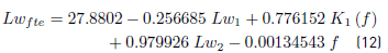
where:
= Sound power level in function of the wind velocity and the frequency, dB(Z)
 = Parameter as a function of frequency, dB(Z)
 = Sound power level in function of wind velocity, dB(Z)
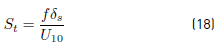
f: Frequency, Hz
The sound power level as a function of wind velocity and frequency is obtained by the Equation. (13):

where:
= Integral boundary layer parameter, m
 = Wind velocity at a height of 10 m, m/s
 = Number of blades
The integral boundary layer parameters are obtained through the Equation. (14) and Equiation. (15) [11]:
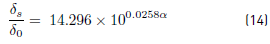
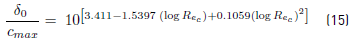
where:
 = Angle of attack
 = Maximum length of the chord of the blade, m
 = Reynolds number
The angle of attack usually varies between 0 ° and 25 °, and because it is a difficult variable to obtain, it can be assumed equal to 15 ° in the absence of values.
The Reynolds number is given by the Equation. (16) [11]:
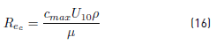
where:
 = Air density, kg/m3
 = Air viscosity, kg/m∙s
= Maximum length of the chord of the blade, m
The parameter as a function of frequency is given by the Equation. (17) [24]:
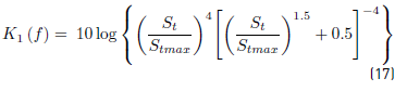
where:
 = Strouhal number
 = Maximum Strouhal number (equal to 0.1)
The Strouhal number is given by the Equation. (18):
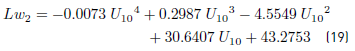
The sound power level as a function of the wind velocity is given by the Equation. (19):
The sound power level due to detachment of the turbulent boundary layer at the trailing edge is given by the Equation. (20):
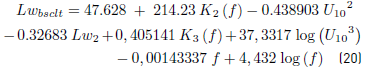
where:
 = Parameter as a function of frequency, dB(Z)
 = Parameter as a function of frequency, dB(Z)
The parameter as a function of frequency is given by the Equation. (21) [24]:
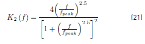
where:
= Peak frequency, Hz
Peak frequency is given by the Equation. (22) [24]:
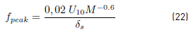
where:
 = Mach number
The Mach number is given by the Equation. (23):
where:
 = Sound propagation velocity, m/s
The parameter  as a function of frequency is given by the Equation. (24):

The sound power level due to detachment of the vortices of the laminar boundary layer at the trailing edge is given by the Equation. (25):
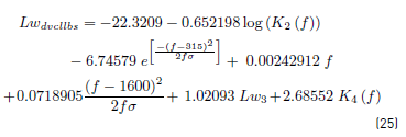
where:
 = Geometric standard deviation of the frequency, Hz
 = Sound power level as a function of the wind velocity and the frequency, dB(Z)
 = Parameter as a function of frequency, dB(Z)
The geometric standard deviation of the frequency is given by the Equation. (26):
The sound power level as a function of the wind velocity and the frequency is given by the Equation. (27):
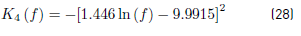
The parameter  as a function of frequency is given by the Equation. (28):
The parameter as a function of the Strouhal number is given by the Equation. (29):

where:
 = Strouhal number
The parameter in function of frequency is given by the Equation. (30):
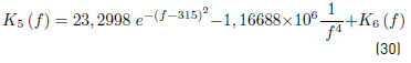
where:
f = Frequency, Hz
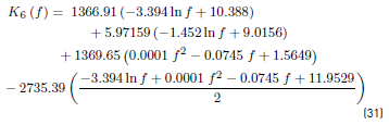
For frequencies ( 500 Hz is given by the Equation. (31):
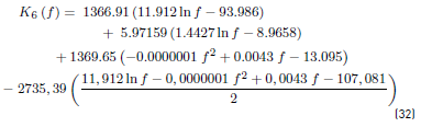
For frequencies ( 500 Hz is given by the Equation. (32):
The parameter of wind velocity is given by the Equation. (33):
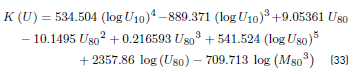
where:
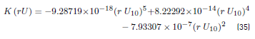
 = Wind velocity at a height of 10 m, m/s
 = Wind velocity at a height of 80 m, m/s
 = Mach number at a height of 80 m
The parameter in function of distance is given by the Equation. (34):
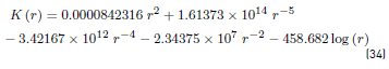
where:
 = Distance between the wind turbine and the receptor, m
The parameter as a function of distance and wind velocity is given by the Equation. (35):
The parameter as a function of the air properties is given by the Equation. (36):
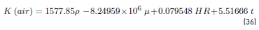
where:
 = Air density, kg/m3
 = Air viscosity, kg/m∙s
 = Relative humidity, %
 = Ambient temperature, ºC
4. Results
To check the accuracy of the prediction model developed, the measured sound pressure levels and the estimated levels were compared. The results generated by the model are as follows:
R2: 92.5 %
R2 (adjusted): 92.4 %
Standard error: 3.8 dB
Absolute average error: 2.9 dB
p-value: 0.00
Four main data sets were used to validate the dependence of the different parameters (atmospheric stability, wind speed, distance and frequency). Since the p-value in the variance analysis is lower than 0.05, there is a statistically significant relationship between the variables at a 95.0% level of confidence. The R2 statistic indicates that the fixed model explains 92.5% of the variation in the residual sound pressure level.
After eliminating the 5.0% of data considered atypical due to their having studentized residuals greater than 2, the fixed model explains 94.7% of the variability in the residual sound pressure level and has an average absolute error of 2.1 dB. The studentized residuals measure the divergence of the observed residual sound pressure levels from the adjusted model using all the data and using standard deviation as a criterion.
A dimensional analysis (using the Buckingham pi method) was also performed in an attempt to reduce the number of physical magnitudes in the form of independent variables that intervene in the description of the phenomenon of sound propagation with the aim of gaining a new insight into its solution.
The method indicated the Strouhal number as an important non-dimensional parameter. This parameter was taken into account in the multiple regression given that the obtained p-value was less than 0.05. This indicates that this term has a statistically significant relationship with the attenuation due to atmospheric stability at a 95.0% confidence level. However, it was not possible to reduce the number of independent variables.
The residual for the wide band equivalent continuous sound pressure level varies between −15.0 and 14.1 dB(Z), with a median of 2.2 dB(Z). When the wide band equivalent continuous sound pressure level is expressed in dB(A), the residual varies between −15.0 and 14.7 dB(A), with a median of −1.9 dB(A).
It is observed that, in general, the lowest values for residual sound pressure levels are obtained by low wind velocities and in stable conditions. In addition, the average residual sound pressure level increases as the frequency increases.
Table 4 presents the difference between the estimated and measured levels for sound pressure variations, both in wide band and with Z and A-weighting filters, for both the proposed propagation model and the ISO 9613 model in its original version. It may be seen from the table that the proposed propagation model is more accurate than the method from the standard ISO 9613 Part 2, especially when the wide band equivalent continuous sound pressure level is calculated with an A-weighting filter.
Table 4 Differences between the measured and estimated sound pressure levels, both in wide band and with A-weighting filters
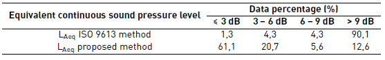
Table 5 presents the statistics for the difference between the measured and estimated sound pressure levels, both in wide band and with Z and A-weighting filters, for both the proposed propagation model and the model from ISO 9613 in its original version.
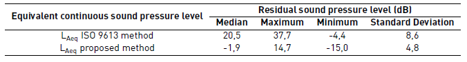
In Table 2, it may be observed that the proposed propagation model exhibits lower median and standard deviation in residual sound pressure level than the method from standard ISO 9613 Part 2, especially when the wide band equivalent continuous sound pressure level is calculated using an A-weighting filter.
5. Discussion
As a result of an exhaustive exercise involving measurement and analysis, the authors propose a semi-empirical model for calculating sound pressure levels at various distances for noise originating from elevated noise emission sources as is the case with wind turbines, which more accurately predicts the actual data or at least comes much closer to doing so. The results have provided a rather satisfactory model to predict noise from wind turbines up to distances of 900 m, greatly improving what has been achieved so far by the method established in the standard ISO 9613 Part 2.
New focuses were used with reference to several specific parameters in noise propagation with the aim of improving the prediction of sound pressure levels or at least to bring them into closer conformity with the actual situation. The reality is very complex, and analytical methods have their limitations. The proposed model offers a compromise between simplicity and accuracy in the prediction of sound pressure levels associated with a noise emission source.
The developed model is well-defined and relatively easy to use. It may be considered a “sub-model” or variation of model ISO 9613 Part 2. As long as the suggested adjustments are applied to the model proposed standard ISO 9613 Part 2, the estimated sound pressure levels exhibit a much better fit with the measured levels.
The number of parameters is greater as compared to the basic components of the model established in the standard ISO 9613 Part 2. Most of the model’s entry parameters are similar, whereas others have been made more complex, resulting in a much more precise model. The basic parameters of the model include distance, height and sound power level of the noise source, wind direction and velocity, and air temperature and humidity. Some of the most complex entry data from the model include ground absorption, atmospheric stability, and directivity factor.
Some of these parameters are more influential than others. The main parameter is atmospheric stability. The second is wind velocity, which affects both the sound power level of the wind turbine and the noise propagation.
6. Conclusion
A statistically significant relationship exists between the variables with a confidence level of 95.0%. The model explains 92.5% of the variability of the residual sound pressure level and has an average absolute error of 2.9 dB. After eliminating 5.0% of the data considered atypical, the proposed model explains 94.7% of the variability of the residual sound pressure level, with an average absolute error of 2.5 dB.
The proposed propagation model exhibits lower median and standard deviation in residual sound pressure level than the method from the standard ISO 9613 Part 2, particularly when the wide band equivalent continuous sound pressure level is calculated using an A-weighting filter.
The residual sound pressure level given by the proposed model is small compared to that from the method established by standard ISO 9613 Part 2, particularly when the distances involved are taken into account. It may be concluded that the proposed sound prediction model is more than adequate to use with a source located a considerable distance above ground level.
In keeping with the above, the atmospheric stability must be taken into account both during measurement and modeling of the noise associated with wind turbines. The proposed model considers atmospheric stability using stability classes and both vertical and horizontal propagation coefficients, which are shown to be more relevant for distances equal to or less than 200 m between the source and the receptor.
Atmospheric stability plays an important role in the propagation of noise, which originates from wind turbines. As one would expect, stable conditions occur primarily at night, whereas unstable conditions have a higher probability of occurring during the day. The experimental data reveal a general tendency of increased stability during the night.

