1. Introduction

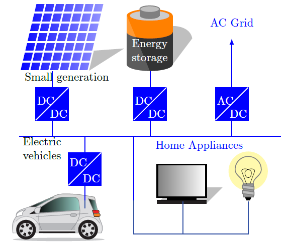
Microgrids promise to play a fundamental role in the future of the smart grid concept specially due to the increasing use of electric vehicles (EVs). This new paradigm allows integration of different technologies with high efficiency and reliability [¹, ²]. In particular, dc microgrids is gaining an increasing interest due to its advances in terms of efficiency, simplicity and usability [³, ⁴]. A dc microgrid can integrate not only EVs but different components such as small scale generation (e.g wind, solar), energy storage and conventional loads as shown in Figure 1. This technology offers advantages such as: i) reduced losses and higher efficiency due to absence of reactive power [³], ii) simplified control i.e reactive-power and frequency controls are not required, iii) high reliability due to its capability of island operation and iv) simple integration since many generation and storage technologies are already dc (i.g solar photovoltaic, batteries). In addition, most of the home appliances could be adapted to operate in dc [⁵].

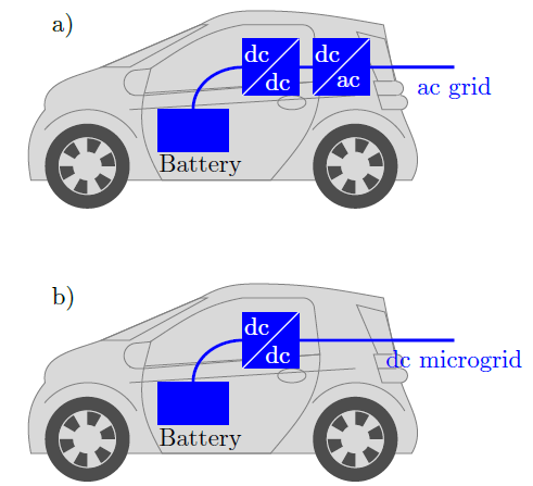
EVs are usually connected to the main grid via two-stage conversion system namely ac/dc rectifier and dc/dc converter as depicted in Figure 2(a). The dc/dc converter is used to control charge of the battery while ac/dc converter is only required for integration to the conventional ac grid. Nevertheless, dc microgrids can be used for optimal integration of electric with a reduced number of components (see Figure 2(b). In this case, efficiency can be improved due to the reduced number of components as well as the aforementioned advantages of dc grids [⁶]. It is required to adapt standard power systems methodologies, such as small signal stability, to this new context [⁷]. The small signal stability is intrinsically related to the characteristics of the network as well as the type of control of the converters [⁸]. In regard to the first aspect, the model of the grid is composed by passive elements (RLC). The control, however, could be different according to the components which are integrated to the grid and the desired operation features of the entire microgrid [⁹].

Figure 1 Schematic diagram of a dc microgrid 

Power electronic converters must be also included in the model since most of the components require to be controlled though such type of devices (ac/dc or dc/dc).

Figure 2 Integration of EVs to the grid a) conventional ac grid b) dc microgrid 

This paper proposes a small signal stability analysis for dc-microgrids considering high penetration of renewable energy and electric vehicles. The main contribution of the paper can be summarized as follows: i) a general model of dc microgrids which includes the dynamics of passive elements as well as the converters according to the type of control, ii) a methodology that includes four operation modes: constant voltage, constant current, constant resistance and constant power with drop control, iii) a small signal stability methodology for the analysis of this general dc microgrid and iv) some general features of the dc microgrid based on the intrinsic characteristics of the model.

It is important to notice the proposed methodology search for a generalized modeling of the terminals under the four aforementioned operation modes. It includes a wide range of applications besides EVs. A small signal stability analysis in a dc microgrid require four steps namely: 1) to pose an acurate but efficient model for the grid and its components 2) to find the operative point 3) to linearize around this operative point, and 4) to analyze the state matrix for the linearized model.

The rest of the paper is organized as follows. In Section II, the main components of the dc microgrid are presented. The model of the converters and their operation mode are presented in Section III. Next, in Section IV the small signal stability is studied. Some general and particular features of the dc microgrid are also described in that section. After that, in Section V, different cases of microgrids are studied with numerical results. Finally, Section VI presents the conclusions followed by the bibliography.

2. Dynamical Model

2.1 Dynamical model of each component

In order to study the stability of a dc microgrid, it is necessary to define a general model for each type of component or terminal. Four type of terminals are considered in this paper for a general description of a dc microgrid. Most of the components are integrated thought a power electronics converter which can be controlled by local regulators with different control objectives, namely: constant voltage, constant power or constant current. In addition, a constant resistance is considered for loads which does not require a converter to be integrated to the dc microgrid. These four type of terminals represent a wide range of possible components and technologies.

Constant voltage terminals are required in strategies such as the master-slave [²] where one terminal fixes the voltage and the other terminals control the power. A constant voltage terminal is usually a generation resource with high power/frequency regulation capacity. It can be also a power electronic converter that integrates the dc microgrid with an AC grid. Line capacitance is not required in the model of this type of terminal since it becomes redundant in parallel with the voltage source.

Constant power terminals include different type of generation resources such as photovoltaic and wind energy, as well as controlled loads [⁹]. These are perhaps the most common type of terminals in microgrids. They are usually complemented with a droop control which enables to run in parallel and specially in island operation, so that total load is shared among generators in proportion to their power rating.

EVs can be modelled as constant power terminals or as constant voltage terminals according to the charge/discharge strategy. In addition, the use of vehicle to grid technologies (V2G) allows a bidirectional value of the constant (P or I). The model of the converter depends on the type of control and not the converter itself. Details of the internal controls can be included in the model although our objective is to maintain a simple and general formulation.

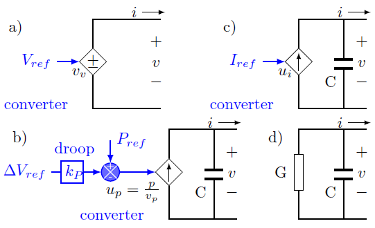
A general model for each of these four type of terminals is depicted in Figure 3. This is a non-linear model due to the constant power loads. Each terminal could be a generation or a load. The difference between them is just the direction of the current. The capacitance C includes the capacitance of the converter and adjacent cables as explained in next subsection. Capacitance in the constant voltage terminal is not required in the model.

Figure 3 Types of terminals in a generic DC microgrid. a) voltage control b) power control c) current control d) constant resistance 

2.2 Dynamic model of the network

Among this section, capital letters represent matrices and vectors, calligraphic letters represent sets and lower-case letters represent one-dimensional constants or variables.

Let us consider a dc micro grid as a set of buses represented by N = {1, 2, …, N}. Each bus of these buses is classified according to the type of control: P node for constant power, I for constant current, V for constant voltage and R for constant impedance. In the two first cases, the node can be a generator or a load. The difference is given by the sign of the reference signal.

The second case is only for generators and the last case is for loads. Let us also define a subset M ∈ N which contains the nodes with a converter (i.e M = N / R).

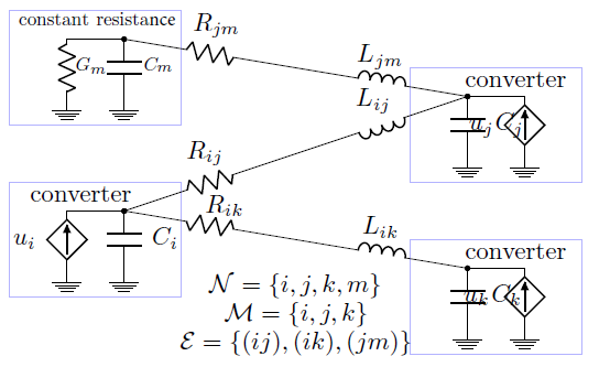
Each line segment (ij) is represented by a set of edges which contains exclusively inductive and resistive elements as depicted in Figure 4 for a four nodes dc microgrid. Branch and nodal variables are related by the branch-to-node oriented incidence matrix :

Figure 4 Diagram of a dc microgrid with four terminals and three converters  

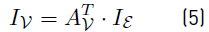
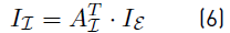
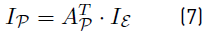
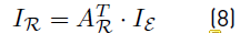
directions and polarity of each nodal current IN and voltage VN are given in Figure 3. This equation can be separatexd in order to analyze each type of terminal independently:

The dynamics of each line segment is given by

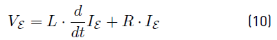
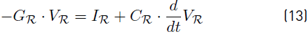
where 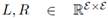are diagonal matrices which represents inductive and resistive effects on the branches. L must be non-singular.

Dynamics of each node is obtained by using the first Kirchhoff law:

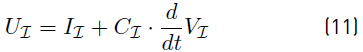
Where C are diagonal non-singular matrices which include the capacitance of each converter and the capacitive effect of the connected line segments. G is a diagonal matrix which represents the constant impedance in case of a constant impedance load. Notice that G can be singular (for example, a step node has gkk = 0).

Control on the constant power loads is represented by a drop regulator as follows:

Notice this is the only non-linearity of the model.

3. Stability Analysis

3.1 Operation point

The operation point is determined by a simple load flow using a Newton-Raphson methodology. Let us define the admittance matrix as follows

were R, A and G are the matrices defined in the previous section. Notice that Y is positive semidefinite and that the effect of constant resistance nodes were included in the matrix Y. Therefore it is possible to make a Kron elimination resulting in a reduced matrix as given in (17)

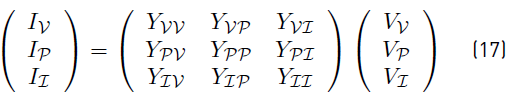
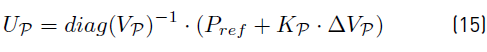
where II and VV are given values (i.e Iref and Vref respectively). In addition, it is required to consider (15) for the constant power terminals resulting in a non-linear system. A Newton-Raphson methodology is proposed for these terminals with the following Newton iteration:

where the superscript denotes the iteration and the Jacobian J(VP(k) ) depends on F, D which are constant matrices as follows

Once the methodology has converged, it is possible to calculate the remaining voltages an currents as follows:

Notice that there must be at least either one terminal of constant voltage or one terminal of constant current. Otherwise the Jacobian in (18) would be singular. The Newton-Raphson methodology is only required for constant power terminals. The operation point in a dc microgrid without those type of terminals can be determined directly from (17).

3.2 Small signal model

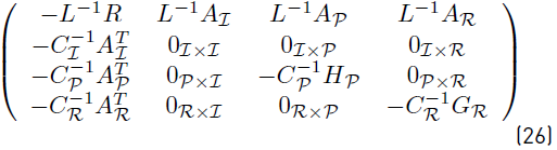
The non-linear dynamic system is linearized around the operative point resulting in state matrix given in (26)

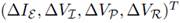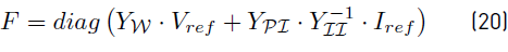
with state variables given by and H _P obtained as follows:

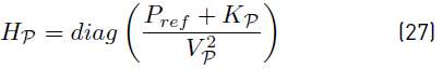
The state matrix can be used to analyze the stability of the entire dc microgrid. Zero matrices are accompanied of a subscript to indicate their size . Notice that some terms of the state matrix depends on the operation point (e.g the block matrix HP). The relation between drop control and active power is clear in this expression.

4. Homogeneous grid with EVs

Let us analyze a homogeneous microgrid without constant power terminals. In this type of microgrid, the cross sectional area of the cable is the same for each line segment and hence, we can define a constant1 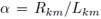. Notice that length of each line segment can be different and hence, Rkm and Lkm are different although is the same. The graph which represent the grid must be connected. Although this case is very restrictive, it gave some interesting results that deserve to be analyzed before presenting results for the general case.

The state matrix for this case is given by

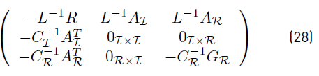
Notice that the operation point does not influence the stability of this type of microgrid. In addition, for homogeneous microgrids, matrix 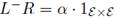where former term represent the identity matrix.

¹We do not make any assumption about whether this constant is high or small

Let us consider the right eigenvectors ϕ and the eigenvalues of (28) as follows:

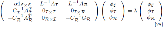
Using straightforward algebraic manipulation and assuming λ≠ 0, we can write this as

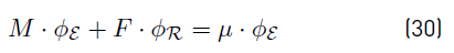
With

Notice that M is a negative-definite matrix since and are laplacian matrices, and L is a diagonal positive-definite matrix. If GR = 0RxR then µ is the eigenvalue of M (which is negative). Therefore, we can obtain the eigenvalues λ for this particular case

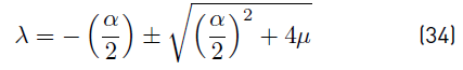
The system is oscillatory if any . In that case the eigenvalues λ are alined with a vertical line in . On the other hand, it is obvious that implies for the non-oscillatory case. Consequently, the grid is always stable regardless the operation point.

Let us now include the constant resistance terminals. In that case the system is obviously stable since G _R is negative-semidefinite. In fact real(λ _R ) ≤ real(λ) where λ _R are the eigenvalues of the system with constant resistance terminals. This follows from the triangular inequality using the maximum eigenvalue as a norm.

This analysis leads to a general result: homogeneous microgrid without constant power loads is always stable. The only source of instability is hence, the constant power loads as demonstrated in the results below.

5. Results

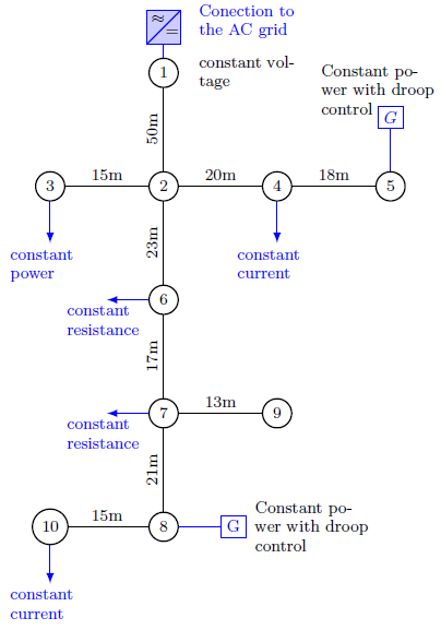
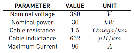
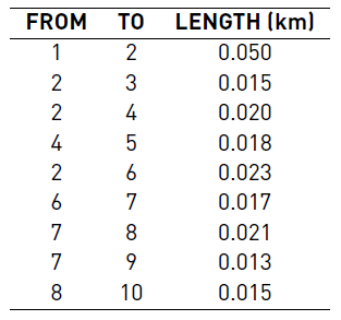
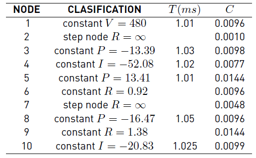
A simulation study was performed on a 380V; 30kW microgrid with the topology depicted in Figure 5. Parameters are given in Tables 1 to 3. In a first case, the cross sectional area of the cable were the same for each line segment and hence the microgrid was homogeneous. The cable is AWG2 of 6:544mm with a maximum current of 96A. Constant power terminals were set to zero in this case.

Figure 5 Graph of the studied microgrid 

Eigenvalues for this homogeneous micro-grid are depicted in Figure 6. First, it was analyzed the case where the constant resistance terminals are neglected. As expected, the eigenvalues were placed in a vertical line given by . Next, it was included the constant power terminals. Eigenvalues moved to the left. This shows numerically the results presented in Section 4 (i.e The homogeneous micro-grid is always stable).

Table 1 General parameters of the microgrid 

Table 2 Connectivity of the microgrid 

Table 3 Clasifications and parameters of each Terminal 

A second study was performed on a more general dc microgrid. Constant power terminals were allowed as well as different cable cross section. The Newton-Raphson algorithm was executed in order to obtain the operation point. It took four iterations with a final error of 7.12 x 10-7. After that, the eigenvalues of the state matrix were calculated. Results are depicted in Figure 7. Eigenvalues are not alined but the average is still an reference which gives some idea about the position of the eigenvalues (see the magnitude of the vertical line in Figure 7].

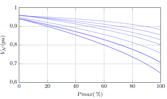
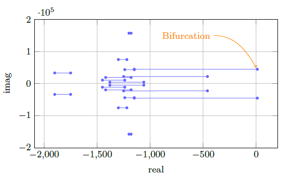
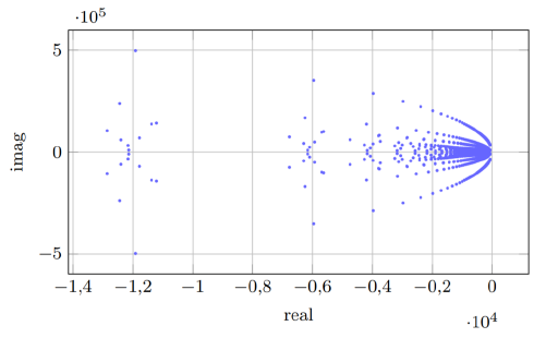
Different values of P _ref in the constant power terminals were evaluated in order to identify possible unstable operation points. This reference power was increased constantly and plotted versus the terminal voltages as depicted in Figure 8. Voltages decreased monotonously until a minimum admissible voltage. Notice the similitude with voltage stability studies in power systems. Each operation point generated a different set of eigenvalues which were plotted as shown in Figure 9. The maximum allowed voltage correspond to the Hopf bifurcation where the system losses stability.

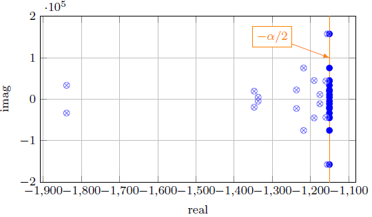
Figure 6 Eigenvalues for the homogeneous micro-grid: (b) without constant power terminals and (a) without constant power and resistance terminals  

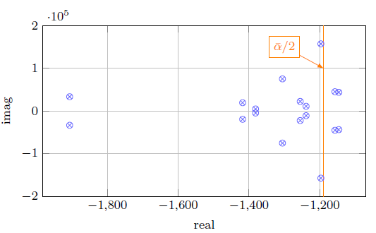
Figure 7 Eigenvalues of the proposed dc microgrid with constant power loads and different types of cables  

Figure 8 Voltages in each node for different values of P _ref in the constant power terminals  

Figure 9 Eigenvalues for different values of P _ref in the constant power terminals 

A sensitivity analysis was also performed. First, it was studied the variations of the oscillations modes respect to the inductance in each segment of line. Results are depicted in Figure 10. A variation on this parameter resulted in a movement of the complex eigenvalues in direction to zero. However, the grid never losses stability.

Figure 10 Root locus of the system for different values of L 

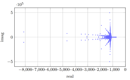
Next, the sensitivity respect the capacitance was studied. In this case, a vertical movement of the complex eigenvalues was observed as shown in Figure 11. The grid remains stable.

Figure 11 Root locus for different values of C 

6. Conclusions

A general model for small signal stability in dc microgrid was presented. This model included the dynamics of passive elements as well as the dynamics of the power electronic converters. Three type of terminals were considered namely: constant power, constant voltage, constant current and constant resistance. Drop control control was also considered in the model for constant power terminals. These comprise most of the type of terminals and controls for dc microgrids.

In the homogeneous case (i.e. a microgrid with an unique type of cable) the eigenvalues were placed on a vertical line around . The system is always stable in this case. For the heterogeneous case this result was not general although the eigenvalues tended to be around an average . Complex eigenvalues were highly influenced by the capacitive and inductive effect of the grid. Power in the constant power terminals was the main source of instability in the dc microgrid. However, the Hofp bifurcation is achieved at very high values showing that, in general, dc microgrids are very stable.