


 English (pdf)
 Article in xml format
 Article references
 Send this article by e-mail
 Cited by SciELO
  Cited by Google
  Similars in
SciELO
Similars in
SciELO  Similars in Google
 Permalink
1. Introduction
Engineering materials are generally subjected to different types of stress or loads. In these cases, it is necessary to know the technological characteristics of the material, in order to calculate and evaluate in the design process, the stresses, and strains to ensure the functionality of the parts.
The mechanical behaviour of a particular material reflects its response to the application of a load. Therefore, the mechanical properties are those characteristics of a material, which are associated with an elastic or inelastic reaction when a force is applied, or relating the relationship between stresses and strains. In the process of product development, the design stage requires thorough understanding of the mechanical properties. At this stage, from the service destination of the part, the most suitable materials for different applications are selected, considering the mechanical properties that allow them to respond to different stresses. In this design process, the behaviour of machine elements and structures are predicted, determining general and specific dimensioning. As important considerations, it should be observed the recommendations for finding the most economical and environmentally friendly solutions. In several engineering applications, the effects of resilience and toughness are currently not explicitly taken into account in the design and construction of welded thick plate joints under high loads or dynamic behaviour.
Therefore, this area of research has recently received attention from the research community. In the most recent studies, it is appreciated a strong interest in finite element modelling as an alternative tool for effective behaviour analysis of welded joints. The numerical method has the advantage of complementing the experimental method, in reducing costs and ease to perform the parametric studies attached to the CAD-CAE systems.
Several authors have explored the determination of the toughness of the materials by different methods. Noguera and Miró [1] determined an asphalts toughness by means of tensile test to relate it with the fatigue test results. García et al., [2] used the fracture toughness of advanced high strength steels (AHSS) to optimize the crash behaviour of structural components. In [3] Gutierrez et al., proposed a new methodology for estimating the fracture toughness by means of Small Punch Test specimens with a longitudinal non-trough notch, which was tested on a 2.25Cr1Mo0.25V steel. The results show that the test requirements are met and they also show the clear influence of notch radii on the measured values. Meanwhile, El-Hassouni, Plumier and Cherrabia [4] presented experimental and numerical results of dynamic cyclic tests carried out on two specimens of welded beam-to-column connections. The analytical results obtained from the numerical simulation predict well the structural dynamic behaviour up to failure of welded connections, compared with the experimental data.
Recently, Tong et al., [5] focused on the fatigue failure behaviour by means of experimental study and finite element analysis, in beam-to-column welded joints under earthquake action. The predicted load displacement response agrees well with the test results.
In a research conducted by Zhang, Xia and Yuan [6], the researcher carried out a series of tensile tests, and used the 3-D finite element models of tensile specimens to analyse the influences of different yield functions upon evaluating several engineering relationships. The comparisons between the simulations and the experimental results show a good solution to found predictive models. Tawfik et al., Islam et al., Chin-Hyung et al. and Wang et al., [7-10] obtained similar findings. In another research, Se-Yun et al., [11] predicted the residual stress distribution produced by electrogas welding (EGW) joints, through a computational approach considering moving heat sources. The residual stress profiles determined by the FEA and the measurement showed quite a good agreement. A nanoindentation, tensile test, finite element analysis, and an optical microscopy was used by Thai-Hoan and Seung-Eock [12] to investigate the mechanical properties in an SM490 steel welded zone. The study concluded that the nanoindentation with the aid of finite element analysis provides an appropriate approach for determining the basic mechanical properties of a structural steel welded zone. The plasticity-based distortion prediction method to address the computationally intensive nature of welding simulations was improved by Yu-Ping and Badrinarayan [13]. To enhance a welding sequence to control distortion, the authors proposed a new theory to consider the effect of welded interactions on plastic strains. The method was validated with experimental work and tested on welded structures, showing that this method can predict distortions fairly accurately. In the same way, Yooil, Jung-Sik and Seock-Hee [14] present a novel numerical method through which less mesh-sensitive local stress calculations can be achieved based on the 3D solid finite element method.
Diverse authors have used the numerical simulation intensively for the study of the thermo-mechanical behaviour of welded joints. In this direction, Pozo-Morejón et al., [15] described the thermal modelling of the GTAW welding on an AISI 316L stainless steel plate, using a previously developed methodology for 3D nonlinear transient modelling of the welding process. The good correlation obtained among the results calculated by means of the model and the experimental data validates the improved methodology. On the other hand, Damale and Nandurkar [16] conducted a 3-dimensional coupled transient thermal analysis for simulating the arc-welding phenomenon. The thermal model was verified by comparing the macro-graph of Finite Element Analysis model and the weld.
Lee, Chiew and Jiang [17] carried out a numerical investigation on the residual stress distributions near the weld toe of plate-to-plate Y-joints, and Fua et al., [18] investigate the welding residual stress and distortion in T-joint welds under various mechanical boundary conditions, using an experimentally calibrated and sequentially coupled thermal and mechanical 3D finite element (FE) model.
In this paper, in order to obtain a better understanding of the stress resilience and the toughness in welded plates, an experimental and numerical evaluation is carried out. The process used to build the joint was Shield Metal Arc Welding. The material base of the specimens was AISI 1015 steel, the filler was E6013 electrode and the butt welding of plates was carried out by the manual method. The experimental evaluation of the tensile test of the welded joint was accomplished, and subsequently was simulated by the finite element method. Four specimens (two notched) were used. An algorithm that calculates the resilience and toughness is implemented. The algorithm was validated by calculating the resilience by the analytical method and the empirical method. For both cases, the obtained percentage errors are considered allowable.
2. Materials and methods
2.1. Characteristics of materials used to manufacture the welded joint
To make the welded joints, the Shield Metal Arc Welding process was used. The electrode utilized was E6013.
Base material
For the welded specimens, it was used as the base material the AISI 1015 steel, which has good weldability. Chemical analysis was performed on an ARL 3460 quantometer to an square sample (50 mm of side and 4 mm of thickness) taken from the base material. In Table 1, the chemical composition obtained is shown.
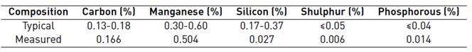
Table 2 presents the mechanical properties of the material. [19]

Filler material
The electrode used was AWS E6013. Table 3 shows the mechanical properties of the weld deposit. In the first column, we can observe the ultimate tensile strength of the weld deposit, which is superior to the base material (referred to in Table 2]. Therefore, the selecting of this electrode was feasible.
Electrode diameter of 3.2 mm was selected and one pass is made for each side of the welded joint. Due to the metallurgical characteristics of the base material, it was not necessary to apply the pre-heating to the plates.

2.2. Tensile test
The tensile tests were performed on a universal testing machine MTS810 US-made.
The specimen was fixed on the headstock of the machine, while the tailstock displacement was applied at a rate of 0.1 mm/s.
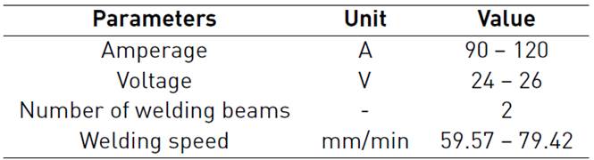
The specimens were made from two steel plates of AISI 1015, abutted by the method of Shield Metal Arc Welding, (SMAW) without edge preparation and welding beams on both sides [Figure 1]. The dimensions of the specimen were determined according to [21]. To determine the parameters of the welding process, a macro called WeldParam was created, employing the Visual Basic for Applications in Microsoft Excel 2003. With this macro, it is possible to calculate the equivalent carbon according to different criteria, the preheating temperature, the welding process parameters as well as other kinds of energy which are important in conducting this investigation. In Table 4, the values of the various parameters of the welding process are disclosed.
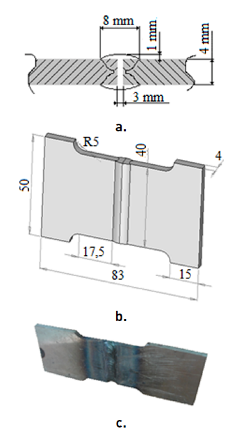
Figure 1 Geometry of the welded specimen: a) Weld bead profile, b) Welded specimen dimensions, c) Specimen welded for tensile tests [22]
2.3. Simulation of tensile test
After carrying out tests to evaluate the tensile behaviour of the specimens, they were simulated through a nonlinear dynamic study using the finite element method. In this model, the definition of constitutive material model and its characteristics is important. The study was developed using the criterion of Von Mises plasticity. They were defined in the software in addition to the material characteristics [Tables 2 and 3], the strain hardening coefficient (n) determined experimentally [Table 7], and the tangent modulus E 1 (according to Equation (1)]. [23]
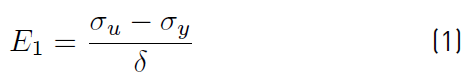
Where:
σu: Ultimate stress.
σy: Yield stress.
δ: Elongation.
In this way, the tangent modulus E 1 equals 269 MPa and 195 MPa for the base material and the filler, respectively.
Geometric model to simulate the tensile test
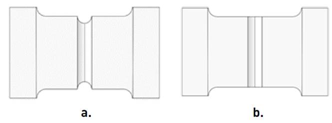
Geometric models used to perform numerical simulations of tensile test are shown in the Figure 2. The geometric modelling was performed in the SolidWorks software, and to develop numerical simulations complement Simulation was used. The notch shown in Figure 2a was developed to induce the fail in the filler material.
Loads and constraints applied to the model
MTS810 machines tensile test, facilitate fixing one end of the specimen and at the other end, apply a load gradually that increases over time. This increased load causes a displacement at the end where the load is applied. To numerically simulate this behaviour, in this study the tensile behaviour of the samples requested was simulated by a static load. This load increased from zero to a final value, the latter corresponding to the final value determined in experimental test.
In Figure 3a, time curve associated with the displacement in the T01S test specimen is shown.
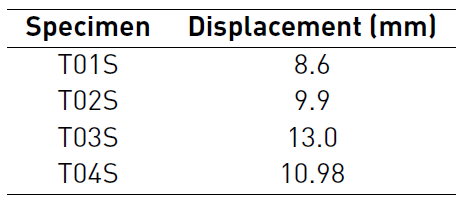
According to the points above, it was decided to simulate this test specimen applying the constraints and loads shown in Figure 3b. At the right end fixed restrictions were applied, considering that the fixed head of the testing machine is on that side. To simulate the tailstock of the machine, it was decided to apply at the left end of the specimen a variable displacement in time from zero to its final value [Figure 3a). For simulated specimens, the final value of displacement is shown in Table 5 (at each simulated specimen, it was added a letter S for the nomenclature).
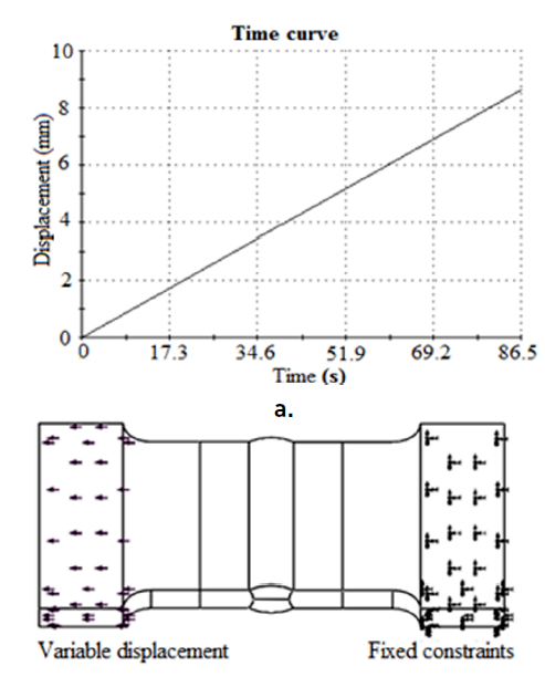
Figure 3 a) Time curve associated with the displacement of the tailstock in the tensile test of the specimen T01S. b) Loads and constraints applied to the specimen
Meshing the model
To perform numerical simulations, a solid mesh was used with quadratic high order finite elements, for best mathematical approximations. Each element was defined with 10 nodes, each with three degrees of freedom, corresponding to each displacement of the coordinate axes.
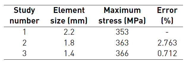
After conducting a mesh convergence study, it was decided to use an element of size 1.4 mm with a tolerance of 0.07 mm. The static numerical study was conducted with a load of 28.5 kN, corresponding to the value of the load in the yield limit of the material. The study results of convergence of the mesh are set forth in Table 6.
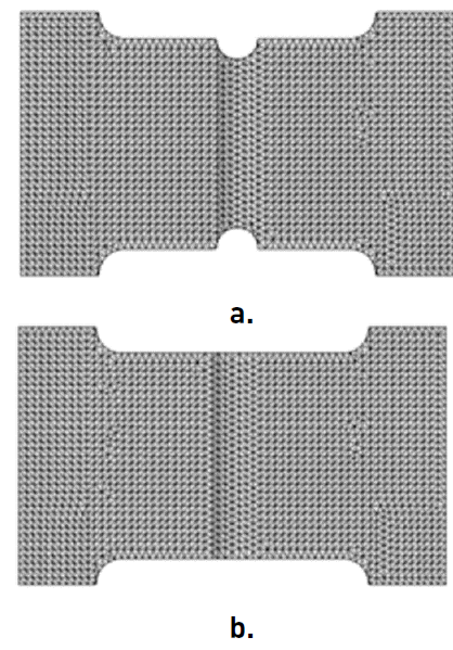
With the size of the finite element used in the studies that was obtained for specimens T01S and T02S, the numerical model has 34,322 elements with 54,488 nodes. For T03S and T04S specimens, the numerical model consists of 34,895 elements and 55,246 nodes. The final shape of the mesh for the different configurations of the specimens are shown in Figure 4.
2.4. Calculation of resilience and toughness for actual tests and simulation
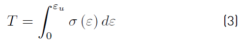
To perform the calculation of the toughness of the tested and simulated specimens, the criterion that the toughness is the area under the stress versus the strain curve to the point where the rupture stress occurs was assumed. Similarly, it was assumed that resilience is the area under the stress versus the strain curve, but only in the domain of elastic strain. [24]Therefore, it is possible to calculate both the resilience (R) and toughness (T) solving the definite integral of the stress versus strain curve (Equations (2) and (3)].
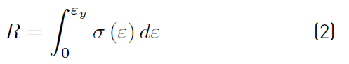
Where: ε y : Strain at yield point,
ε u : Strain to failure
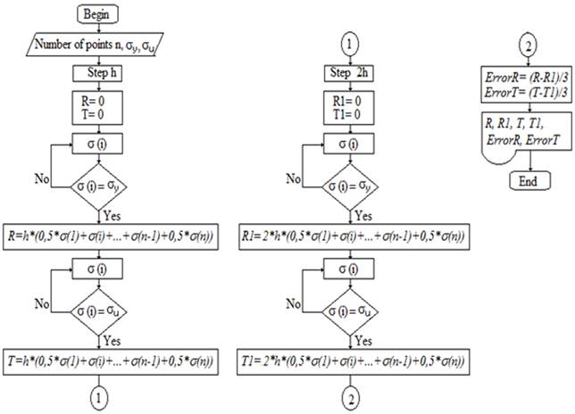
To develop the calculation of the definite integral, an algorithm [Figure 5] which allowed both the toughness and the resilience to be determined using numerical methods was proposed. The trapezoids method [25] was used through the Equation (4) to calculate the area under the stress versus strain curve. In addition, an algorithm also calculate the error occurring in the computation (Equation (5)].
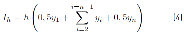
Where: I h : Integral value with step h,
I 2h : Integral value with step 2h,
h: Step,
y i : Ordinate value,
Error: Error method of trapezoids
In the proposed algorithm, the terms R1 and T1 are the resilience and toughness respectively when those parameters are calculated with step 2h.
3. Results and discussion
3.1. Tensile test
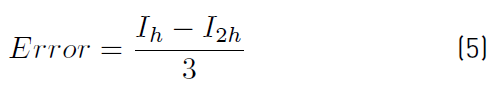
Four welded tensile specimens were tested, in order to know the mechanical properties of the joint. To determine the quality of the joint, it was used as a criterion that the failure of the welded specimen must occur in the heat affected zone (HAZ) and not in the welded metal, demonstrating in this way that the welded joint is well-built. Two of the specimens studied underwent a notch, to assess whether the break occurred in the filler material, which did not happen in any case. In Figure 6, the broken specimens are observed. A specimen on which a notch was performed [Figure 6a), the break occurred in the HAZ adjacent to the change section between the filler and the coarse grain zone of the HAZ. For the unnotched specimen [Figure 6b), the rupture started in the coarse grained HAZ and came after a tear of the specimen that reached the base material. In both cases, it was shown that the welded joint did not fail in the filler, but in the base material.
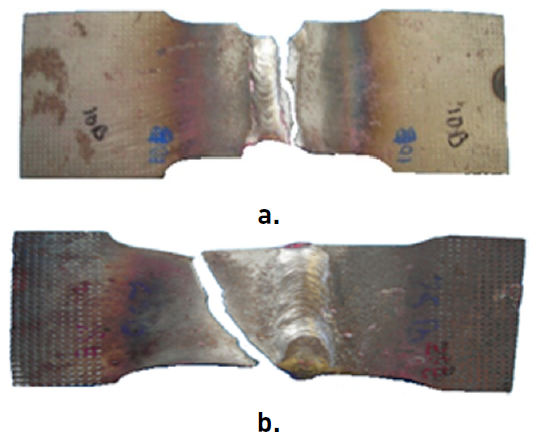
Figure 6 Form of the breakage of the specimens under tensile loads. a) with notch and b) without notch
In Figure 7a, it is shown the graphs of stress σ versus the strain ε obtained from the tests performed at the four specimens, which are denoted as T01, T02, T03 and T04, respectively. It is observed that T01 and T02 specimens (those with indentations) failed before T03 and T04 specimens. Considering that the area under the curve stress versus strain is a measure of the toughness, and then it is possible to argue that the notch applied to the welded joint decreased the toughness. In other way, in Figure 7b are the stress-strain curves for simulated specimens.
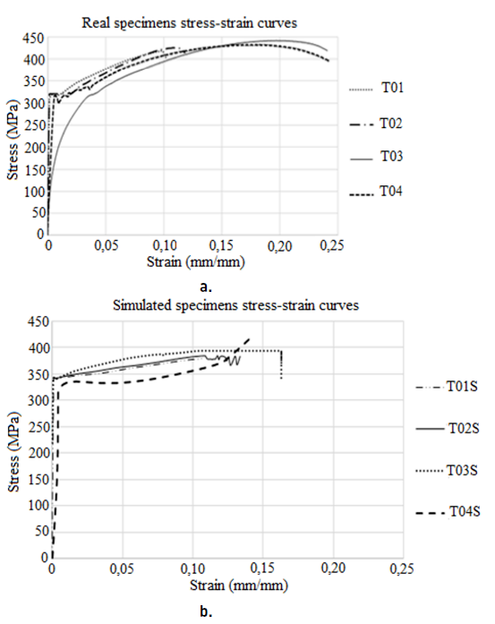
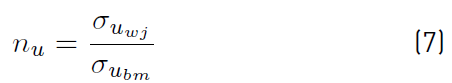
Table 7 shows the values of different parameters determined in tensile tests at welded joints. Efficiency is defined as the ratio of the property of the welded joint and the base material, thereby the efficiencies at yield and the efficiencies at rupture are determined from Equations (6) and (7) respectively. Subscripts bm and wj make reference to the base material and the welded joint, in that order.
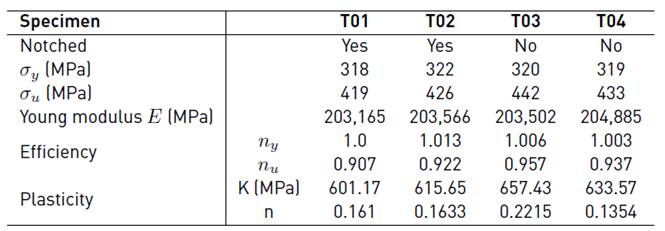
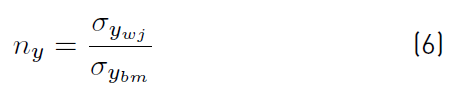
Where: n y : Yield efficiency,
n u : Break efficiency.
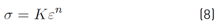
In the same table, the plasticity row refers to the resistance coefficient (K) parameters and the exponent strain hardening (n), to adjust the relationship between the stress and strain in the plastic zone, through a Hollomon type equation (Equation. (8)]. [26]
3.2. Simulation results of tensile test
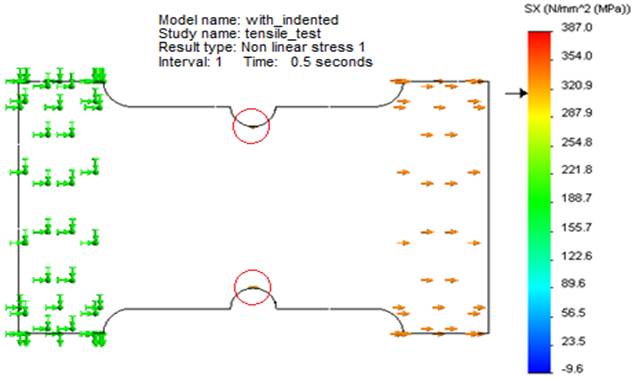
Numerical simulations allowed us to evaluate the tensile behaviour of welded joints. In Figures 8a and 8b, they are displayed at the time of the break (in the last time step), the numerical results of the stress state of the T01S and T03S specimens. In the case of the specimen T01S, the first plastic stresses occur when the displacement is equal to 0.05 mm, and are found in very small zones located in the notch [Figure 9]. The final stress state in this simulated test showed that areas with higher stresses are in the HAZ, precisely in the area where the actual specimen rupture occurred. Hence, the failure occurs in the base metal and not in the weld.
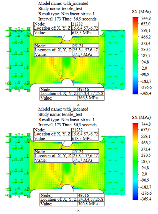
In the case of the specimen T03S, the first plastic deformations occur when the displacement reaches the value of 1.1 mm. These occur in areas situated in the fusion line and parts of the base metal, but mainly in the HAZ. As seen in Figure 8, in the specimen the high values of stress arise. These take place on the transition line and in very small areas. This means that the welded joint failure will occur precisely in the area of HAZ, which is what happened in the actual welded joints.
Measuring the stress and the displacement was conducted in a node located on the fusion line, from the stress versus strain curves obtained by numerical simulation [Figure 7]. As it can be seen, the slope of the elastic portion (Young modulus or modulus of elasticity of the first order) is similar in the simulated curves and in those obtained by experimental tests. In the case of the section of plastic deformation, there are differences in the curves attributable to the fact that the simulation does not occur the plasticity process, the development of micro holes that take place in the tensile test specimens and of course due to the assumed constitutive model of materials.
3.3. Validation of the proposed algorithm
In order to validate the algorithm developed, the resilience was calculated by other methods for T01 specimen. Given the nature of the tensile behaviour of materials, where it is true that in the elastic section the relationship between stress and deformation follows a linear behaviour, it is possible to determine the definite integral as the area of a triangle. The height of the triangle would be the yield limit and the base of the triangle would be the strain up to this limit.
Another way to determine the resilience is by Equation (9). [25]
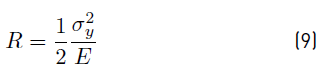
The resilience values obtained using three different methods from the specimen T01, are shown in Table 8. The determined maximum error is 10.12%, which can be considered permissible.
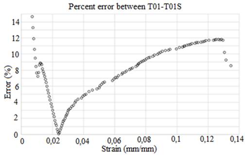
In Figure 10, the percentage error between the samples T01 and T01S is exposed. As shown, the value of the percentage error between the actual specimen and the numerical simulation is never greater than 15%, which can be considered allowable.
3.4. Calculation of the toughness
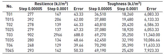
To determine the toughness, the developed algorithm [Figure 5] is applied to all samples studied, both real and simulated. In Table 8, the results obtained for the resilience and toughness in each of the samples are shown.
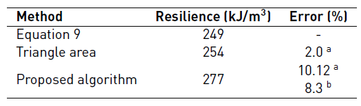
a Regarding the Equation 9
b Regarding the area of the triangle
The above table shows that resilience is similar for almost all samples, that is, they all have the similar ability to recover their original dimensions after removing the load causing the deformation, except for the T03 specimen (the deviation is due to the slope of the elastic portion of the stress versus strain curve). The value of the resilience between real and simulated samples is similar. The biggest difference between the T03 and the T03S specimens occurs because the deviation in the second gradient elastic section of the stress versus strain curve does not occur. The difference can also be appreciated between samples T01 and T01S, because in the simulation, the elastic limit is greater than the actual test. The error calculated by the trapezoids method in the case of calculating the resilience ranges from 14.92% (specimen T03S) and 17.14% (specimen T04). It is observed that in the notched test pieces the toughness is lower than in those where there is no stress concentrator. It can also be noted that the values of toughness between the simulated and the actual samples are similar, except between specimens T04 and T04S.
Noguera and Miró [1] determined the toughness as the area under the force-displacement curve obtained from the tensile test of asphalt mixtures. The results obtained showed that the samples with greater tenacity also had a better fatigue behaviour. It shows the capability to use the tensile test to determine the toughness.
4. Conclusions
This paper presented an experimental and numerical evaluation of resilience and toughness in AISI 1015 steel welded plates joined with SMAW process. By comparing the numerical results which are obtained by simulations versus the experimental results, the following general conclusions can be drawn:
The tensile test of a welded joint butt, using as the base material steel plates AISI 1015 was performed, and as the electrode E6013. The test results provided values concerning the mechanical properties of the welded joint, which were used in the numerical simulation. To perform the numerical simulation a study of mesh convergence was done. It was obtained as a result, a finite element size 1.2 mm a with maximum stress of 366 MPa, with a 0.712 % error percentage. Resilience and toughness for welded joints from experimental and numerical results are calculated. In order to calculate it, an algorithm that allowed us to determine the area under the curve of the stress versus strain curve by the trapezoids method (numerical integration) was implemented. This algorithm was validated by calculating the resilience by analytical methods, obtaining an error percentage of 10.1% with respect to the Equation (4).

