


 Inglês (pdf)
 Artigo em XML
 Referências do artigo
 Enviar este artigo por email
 Citado por SciELO
  Citado por Google
  Similares em
SciELO
Similares em
SciELO  Similares em Google
 Permalink
1. Introduction
1.1 Overall precision in a machine tool
The growing demand for manufacturing more precise large components justifies further development of methodologies to reduce manufacturing time and improve production configurations, in order to achieve quality in the final product [1-3]. Manufacturing large machines requires precision in the assembling of the components, and a larger amount of steel or cast iron, but it is also required to reduce the high cost of manufacture. The current trend is to build machines less robust and more lightweight, therefore their productivity rates are inferior and sensitive to dynamic changes including hardness on the surface of the material [4]. It is noteworthy that each component of a machine contributes to the overall accuracy of the system [5]. Operational errors generated in a machine tool are kinematic, dynamic and thermal [1, 4,6].
Geometric errors in the manufacturing and positioning errors, are responsible for each movement for generating greater uncertainty in the accuracy of a machine [6, 7]. Some investigations have contributed to the development of techniques in the calculation of the minimization of kinematic errors caused by geometric errors of manufacture that influences in the positioning automated machines of 3 degrees of freedom onwards [8, 9]. Guoqiang [10] establishes the geometric errors by a differential motion transformation and are considered as the fundamental pillar theory of robotics. Yang [11] presents a model that allows the kinematic configuration of the machine in the five axes by “Screw” theory. Mostafa [12] recently proposed a new method to identify kinematic errors through a group of probes designed to be measuring error separately.
Loads arising upon contact between the tool and the workpiece generate dynamic errors which are manifested as deformations and vibrations in the machine structure [1, 6]. The modeling system predicts the different phenomena that occur in the structure, and thus the percentage of influence is determined [13]. Yun [14] developed a model for predicting the linear function of grinding force in the orthogonal coordinates X, Y, Z with utility for roughing surfaces of non-homogeneous materials. Park [15] works milling control to determine the optimal inclination of the tool and the forces generated in a preset path.
1.2 Polishing Process
Historically, the polishing process errors were generated by a process performed manually, in which the operator skills were the main parameter [16, 17]. Then, automatic machines and controllers were developed. Preston in 1921, postulated a mathematical model upon the polishing process, based on the material removal rate, according to the relative velocity between the tool and the workpiece, maintaining a constant pressure. It also relates the material mechanical properties of the tool and the lubricating fluid type used in the polishing process. This relationship is known as the primary polishing equation [17-19]. In the 90's, Huisoon [20] presented an experimental study that showed the effects that occurred in the workpiece when varying the configuration of the various polishing parameters using an abrasive disc of steel to determine a certain type of roughness. Liao [16] developed adaptive pressure control to determine when the tool head keeps constant the contact between the tool and the workpiece to ensure the polishing process. Khan [21] presented a mathematical model to estimate the surface residual errors from the operating parameter settings. When the surface has a complex shape, the simple model fails, and the influence function appears [18]. Schinhaerl [19] studied the distribution of material removal in relation to some influence function. Wang [22] developed a prediction model material removal with grinding stones; the relationship between pressure and depth removal is analyzed creating a distinctive profile material removal using Hertzian distribution. Temmler [23] developed an algorithm called selective laser polishing to enhance the surface appearance, through reallocation of material instead of ablation with laser remelting in metallic surfaces. This algorithm is not achieving the flatness and the material is not removed. Algorithm has a great utility to achieve a greater precision in the design of surfaces such as leather textures, automotive panels and the metallic surfaces. In the case of petrous materials, the laser is not useful due to the high energy consumption, so the processes of elimination of material by direct contact must be considered. Hence this algorithm must consider the cutting forces, vibration effects and manufacturing errors that occur at the time that the tool and workpiece are touched.
1.3 Error Compensation
The study of error compensation has been applied to methods since the 70s to correct errors in machine tools [24]. Xiaoyan [8] presented an integrated error compensation model. Integration is accomplished by error propagation based on the Jacobian-Yawing theory. Ahn [25] proposed a mathematical model for error correction in machines with 3 axes of freedom formed by the 21 components of error [7], involving the x, y, z axes for both linear and rotational movements. Abdul [26] introduced a technical error for 5-axis machines establishing 52 positions independent and dependent, which are identified dividing the machine into five rigid bodies by eliminating the configuration errors of the piece and cutting tool. Sortino [2] proposed a new approach to produce a piece with a previously generated trajectory, then the piece is measured to determine the displacements, and finally, shifts are taken to improve.
Identified errors are obtained using specialized equipment such as laser interferometer metrology, electronic levels or autocollimator [27-29]. Alternative modelling techniques to identify errors can be performed using indirect measurement. i.e. nonlinear techniques of volumetric verification, aiming to minimize the difference between actual positions versus the theoretical positions [30, 31].
After conducting a deep research in the literature about the development of this process, this article presents, first, the new method APLM to achieve precision in the polishing process. Second, an alternative method of polishing called Selective Polishing (SP) in the production of the flat surface in petrous materials.
In the next section, this article proposes a solution to resolve different type errors depending on the process to be performed. It also presents how the compensation of the errors is calculated, and finally, the development of the selective polishing is shown from the developed compensation.
2. System Description and Mathematical Formulations
The manufacturing process is accomplished through theoretical and experimental forms. A deductive analysis selects the different processes and interfaces including an inductive validation and the feedback to optimize the result. The development of a machining process of flat surfaces requires a vision of possibilities for the equipment to find different types of errors. Such result is presented as a combination of methodologies and known achievements linked to the contribution of researchers. This validation is performed for the mathematical model and the equipment. The mathematical model of the systems is expressed such as a set of significant errors becoming in functions where input variables must be measurable, i.e. position, velocity, and force arising, due to the grinding and polishing processes.
The methods proposed in this article, first, the adding precision method to the lightweight machines through the identification and the control of the static and dynamic errors, and second, the SP method are expressed with the following equations.
2.1 Static Errors
The first part of the formulation is based on the interpolation method defined by parts which is transformed to define the machine characterization and then, to determine the position of each point in function of x, y, z axes. Each body is analyzed and stored in a position matrix. Figure 1 shows the schematic errors on the reference system, where the deviations, the fabrication errors and the installation errors are illustrated.
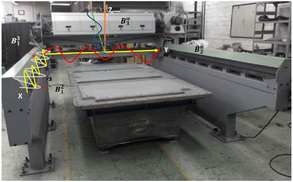
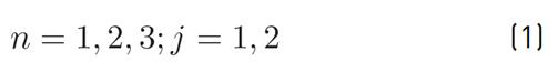
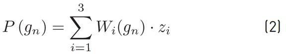
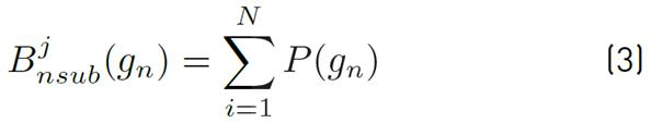
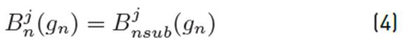
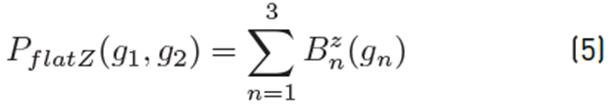
The mathematical formulation of the first part is described with equations (1) - (5). Equation (1) shows the subscripts and superscripts used for the formulation. Subscript n uses 1, 2 to denote the stringers and 3 to refer the movable bridge. Superscript 𝑗 refers to the two polynomial equations per body. In Equation (2),  represents the second order polynomial equations of each structure, Wi(gn) is the multiplier, Zi is the analysis point; in Equation (3), Bjnsub(gn) is the summation of the entire section. The points corresponding to the guide of displacement in relation to the axes x, y, z are denoted as gn. In Equation (4), Bjn corresponds to the bodies of the machine. For Equation (5), the unique polynomial for flatness in Z is obtained through PflatZ in relation to x(z) the values respect to the Z axis are evaluated in PflatZ (g1, g2) and it is stored in a matrix.
Errors produced by static deflection, in relation to the Z-axis are considered, including the effects of the weight of the machine subsystems and of the structure, through Timoshenko’s elastic theoretical formulation [32].
2.2 Dynamic Errors
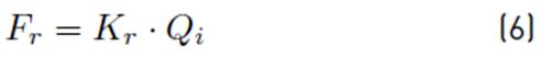
The cutting force of the tool to the grinding process is calculated using the mathematical model presented by Qin [33] (see Equations (6) and (7)]. The force determined from the travel velocity and spindle rotation includes cutting parameters, depths, and specifications of the cutting tool. The model is shown below:
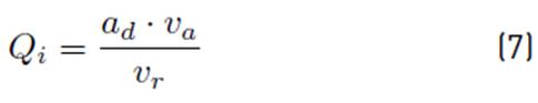
Equation (6) presents Fr, the radial force of grinding process, Kr the specific cutting force, Qi the equivalent chip thickness. The same way in Equation (7), d  the depth of cut,
  feed velocity and v
r
cutting velocity.
feed velocity and v
r
cutting velocity.
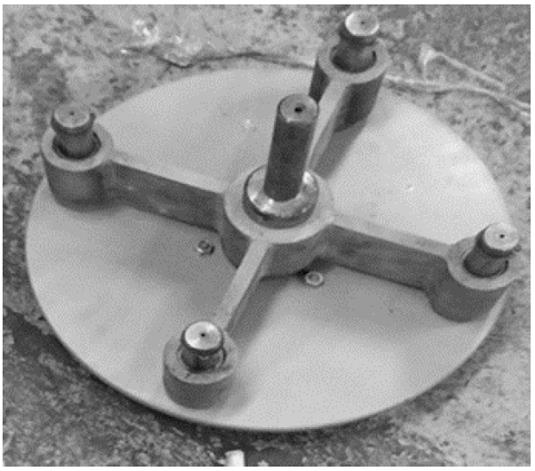
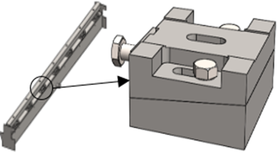
The polishing process was carried out with a specific tool designed to maintain a uniform pressure in the contact area. A disc supported by four columns with springs was used (see Figure 2].
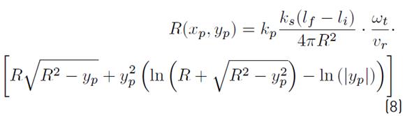
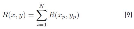
Polishing process is performed following the rectangular path proposed by Lakota [28]. The mathematical model to determine the material removal rate in a point is based upon the law proposed by Preston [18] and Lin [34], which are showed in Equations (8) and (9). Equation (8) presents R(x
p
, y
p
) as the removal rate of polishing material in the position x
p
, y
p
. The work pressure performed is replaced with the four spring constants per unit contact area ,l
f
-l
i
are initial and final string deformations; the relative velocity v
r
between the tool and work surface. The coefficient k
p
parameter called Preston houses the variables concerning the properties of the tool and the workpiece [18]. Equation (9) indicates the total removal material over a given area that is represented as the sum of all points x
p
, y
p
,l
f
-l
i
are initial and final string deformations; the relative velocity v
r
between the tool and work surface. The coefficient k
p
parameter called Preston houses the variables concerning the properties of the tool and the workpiece [18]. Equation (9) indicates the total removal material over a given area that is represented as the sum of all points x
p
, y
p
The total force is housed in the structure F all [N]. It is calculated in Equation (10), as the sum of the forces due to the structure weight F W , to the strength due to the spindle motor F s , and strength cutting tool F C work.

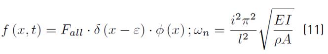
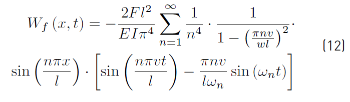
To add stability to a machine, the dynamic structural model having account the grinding and polishing processes is based on the theory of vibrations in continuous media [35, 36]. It presents the (11) and (12). In Equation (11), f (x,t) is the force in terms of the Dirac pulse function ( , the natural frequency (n, E elasticity module, I inertial, ( density, A transversal area, and l the stringers or movable bridge length. In Equation (12), Wf (x,t) parameter is the dynamic deflection due to the force f (x,t). V object velocity along the stringer or movable bridge and n iteration number.
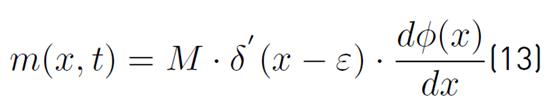
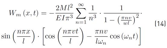
Vibration is considered due to the moments produced by the advancement of the cutting tool, depending on the speed and depth of cut. The mathematical model is based on the formulation set forth by Kozien [37] and it is shown in Equations (13) and (14).
In Equation (13), m(x, t) is the resulting time and the Equation (14), W m (x, t) is the dynamic deflection due to the force that tends to cause rotation M.
2.3 Error compensation
In this article all Z points are evaluated with the above formulations and are introduced in a data matrix with the information that guides the controller in each different situation. The surface of points generated, as result of finding the static and dynamic errors separately, then, these points are saved in the points matrix (PM). In Equation (15), the data acquired of each stringer and movable bridge is stored. To find the Z value the controller receives the sum of the three Z values due to three bodies, for each point X, Y of the surface traversed by the tool; a standard surface with flatness greater than that required for regular production is used. This surface is swept with constants adjustments in the Z axis.

Static and dynamic compensation are performed in relation to the deltas of heights on Z axis. The formulation is presented in Equations (16) and (17).
Equation 16 shows the error compensation static matrix  , it is formed by the ( static static topography matrix and the common pattern topography matrix ( pattern for the formulation of dynamic error compensation. Thus, in Equation (17), it presents the error compensation dynamic matrix
  ,it is completed by the ( dynamic dynamic topography matrix.


2.4 Measurement
The metrology model used is the rectangular extraction strategy of points exposed by Lakota [30]. This formulation is given for Equations (18) to (20).
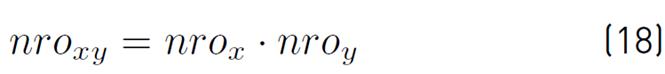
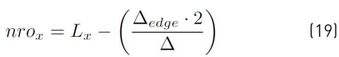
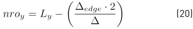
The total number of points nroxy is calculated through of Equation (18); it is analyzed on a surface S. The subscripts x, y are points with respect to the X and Y axes. The definition of the surface S is performed in the X, Y, Z coordinates system. Equations (19) and (20) correspond to the number of points in X and Y for longitudinal and transverse distances Lx/y , these points are measured from the edge to the end of the surface. The measurement separation is called delta (edge . Separation delta ( is the new length on the surface and the first coordinate to measure height Z.
The generation of X and Y coordinate points are obtained through a parametric equation of each line segment, with Equation (21). Where, xi is the new point and the x0 is a known point.
The Z height deltas are taken at each point X, Y with digital precision instruments.

2.5 Selective polishing process
This method to add stability is used to develop the selective polishing process (SPP), this is performed after lifting the matrix of metrology and obtaining the results of the grinding and first polishing process. It is developed to perform the polishing in places of the surface where deltas of heights that are above the range of flatness established were detected. The strategy takes the topology previously measured. In Equations (22) to (28), the mathematical formulation for SPP are presented.
Equations 22 and 23 represent the matrix PM and its dimension.

The Equation (24) shows the infinite norm of the vector  to obtain the maximum value of the column s(:,3) , and corresponds to deltas in Z.

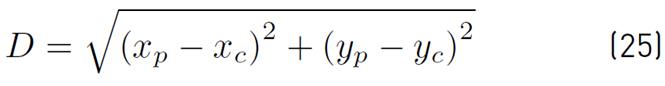
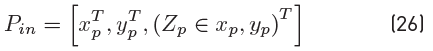
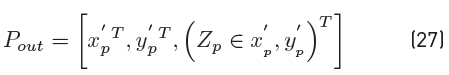
The SPP algorithm works as follows. Firstly, the tool works over a non-polishing area of tool size, and secondly, the points XY-Z that are outside of the perimeter of the circular tool C with radius (r) are known. The algorithm is described by Equations (25), (26) and (27).
In Equation (25), D determines the distance between the points of analysis x p , y p regarding x c , y c central points of the tool machine and depending on the result, with de condition if / else, it establishes the points polished p in and the non-polished p out . Equations (26) and (27) are matrices that store the points that are being analyzed and the missing points analyzed.
The cycle works until the length of the P out matrix is equal to zero.
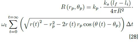
The function of material removal rate for a specific point in Z, was calculated using the Archimedean Spiral Path over the point. This function was introduced by Lin 31. The Equation (28) is expressed as follows.
Where, R(r p ,( p ) is the total removal material, r p goes from the center of the tool to the location point to work for a given time t. The angular velocity (t of the tool. ( p ,is the angle of r p , r , is the distance of the tool center point to initial polishing point, ( is the angle of r
3. Methodology
In this section, a real case of the design and built of a machine to manufacturing flat surfaces of petrous material (see Figure 3) is presented, using a mixed process that combines the classical methods and the new one introduced in the previous section.
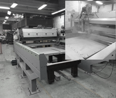
This section describes one by one how the topics were addressed to achieve the behavior of the complete system and its interactions. The selective polishing process, the selected methods, the procedures, the equipment operation, the static-dynamic behavior, and the control system are presented and developed below.
3.1 Procedure to develop the process
This procedure was divided into stages having into account the different methods. These phases were named in the following order: design of the machine, kinematic errors, metrology strategy, errors compensation and grinding-polishing process. The selection is made by means of the following design criteria: large format, integration of subsystems, lightweight structure (not robust), and compensation using machine intelligence in the grinding and polishing processes at the same machine.
3.2 Selection of methods
The identification of the different types of errors was performed with APLM method. This method shows manufacturing, misalignment, installation problems, static and deflection dynamic and the vibration frequencies. It is supported by the fact that each body of the structure has deviations, therefore, the sections are not straight; each body is modeled mathematically through the summation of Lagrange second degree polynomials. Through this certainty each structure is statically and dynamically analyzed separately as a continuum body with its corresponding differential equation; then, each equation is evaluated on n-point chosen; finally, those Z points are computed in the PM matrix in the X and Y coordinate, applies in each Z. First, with respect to the grinding process, the mathematical model to determine the cutting force considering the flat surface in petrous material is the proposed by Qin [33]. Second, the metrological process was performed combining the differential measurement method with digital instrument, proposed by Haitjema [27], and the strategy point extraction route and flat surfaces researched by Lakota [28]. Third, the polishing process was carried out by mixing three methodologies. Fourth, the law of Preston [18] for calculating material removal per pressure, fifth, the methodology of path planning proposed by Lin [34] and a strategic proposal in this research. And the last the SP method.
3.3 Manufacturing process
In this section, the article presents the way in which the machine works and how the flatness in the petrous material is achieved. The process is described below.
First, the tool passes to a fixed height using a coarse-grained abrasive (80-120). Secondly, the topographic map of the surface is made by measuring instruments. The third step, the method of selective polishing uses fine abrasive stone (600 grit) is made. Finally, metrology is performed to save the work and traceability.
3.4 Static compensation process
The measured points are the input data for the correction, then, with the metrology of the pattern surface and the state of the machine, the compensation of the machine is performed by means of a computational algorithm considering the phenomena that are generated and that the application must solve.
Due to the load points and the weight of the structure, misalignments, manufacturing errors, deflections of the beams and the bridge were introduced to generate a static flatness. Static topography at any point on the surface is calculated in the algorithm by 2D interpolation through the cubic approximation.
Mechanical leveling
To improve the static linearity of the guides, mechanical levelers in the stringers and the bridge of the machine were added. It allows the fabrication errors of the machine are compensated (see Figure 4]
3.5 Dynamic compensation process
The dynamic correction values consider the path velocity, the cutting force of the tool, the material removal rate, and natural frequency of the system. Similarly, as in the static topography, the dynamic analysis for grinding work and continuous polishing are stored in a matrix with coordinates X, Y to the path generator.
The final flatness calculation is described by Equation (29). This process finishes when the error value with respect to the pattern surface is less than the agreed error.

Error of acceleration and deceleration of the system
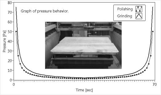
Experimentally, for continuum grinding and polishing process, the acceleration and deceleration during the tool path on the workpiece affect the flatness of the working surface (see Figure 5], generating higher pressures producing a higher material removal rate in these places. The distribution of tool pressures on the surface for acceleration and velocity changes must be determined because these facts affect the quality of the flat surface.
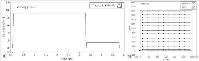
The optimization of the material removal establishes relationships between the translational velocity of the tool and the angular velocity of the spindle, to generate a less trapezoidal velocity profile (see Figure 6a) and maintain the equal removal rate over the entire surface, both in the edge area and also in the middle area as shown in Figure 6. In Figure 6b, the changes in the velocity of the spindle (rpm) in relation to the position of the tool along its path can be seen.
The tool does not leave the work surface during the path; the reason for this is that the normal force exerted by the surface to the tool, it causes the lifting of the bridge resulting in the cut of the tool to be irregular, and step-shaped waves appear.
3.6 Selective Polishing process
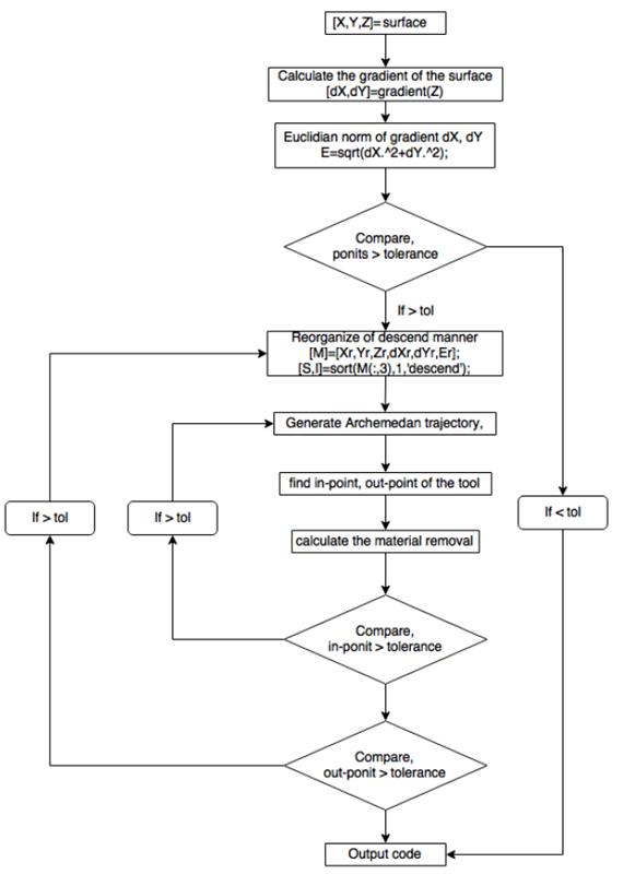
This process is organized in a closed loop for rectification work, metrology, selective polishing and final metrology certification to meet the range of proposed flatness. The following figure shows the schematic diagram of processor software for selective polishing (see Figure 7]
With the results given by the algorithm, a controller is loaded with the data that includes the compensation of each position X, Y for the Archimedean Movement, the angular velocity of the spindle, the compensation in the Z axis, and the mechanical properties. The parameter  is considered to determine the material removal rate in each zone to achieve the flatness required.
3.7 Control systems
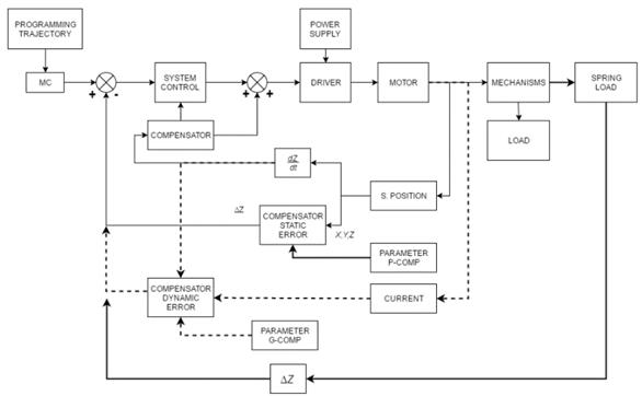
In grinding and polishing processes, it is established the following control systems configurations for positions X, Y, Z coordinates as inputs for the compensator error (see Figure 8].
The control system for the grinding process [Figure 8] initializes with the path programmed associated with a movement control that delivers the desired positions X, Y, Z. Then, the controller energizes the electric motors which, in turn, provides the output mechanical energy to a movement converter from the rotational to linear. From the motor, the positions signal and current (torque) are obtained. For the static compensator, the position signal corresponds to the motor signal, while for the dynamic compensator, the signal input of velocity is the derivative of the position Z to obtain the dynamic behavior. The position correction is achieved. First, by manipulating the torque signal that is converted into an amplified current signal, second, by obtaining the physical and mechanical parameters of the machine and the workpiece, third, by taking the values in a package of data and entering them to the dynamic and static compensators provided by the offset of the control, and finally, doing the comparison with the deltas Z to make correction.
Once programmed X, Y, Z coordinates, the compensation for the selective polishing is performed similarly to the grinding process, as this has the same compensating for static error. However, for this compensation,  changes with the error in the surface and it is indicated in the position sensor. The pressure is generated by the force of the springs that push the tool against the surface i.e. When the controller does not perform a corrective action, the polishing process is carried out at a variable pressure, only depending on the stiffness of the springs.
4. Result
4.1 Validation of the method
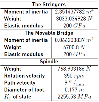
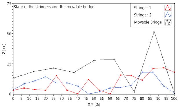
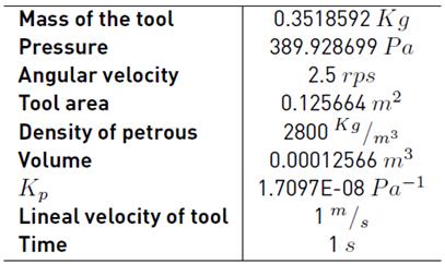
The flatness measurements were performed using electronic equipment on the petrous material to establish the tolerance. Then following machine parameters were established; mechanical properties and operating data (see Table 1]. Finally, the topography of the structure through data discretization was obtained to establish the degree of leveling in the stringers and the movable bridge. These results are shown below.
Deductive result is achieved through measure equipment of high precision and the method described knowing the state of the pattern surface (PS) shown in Figure 9; this flat PS (2x1.6m) has an error tolerance of ±10µm .
4.2 Static compensation process
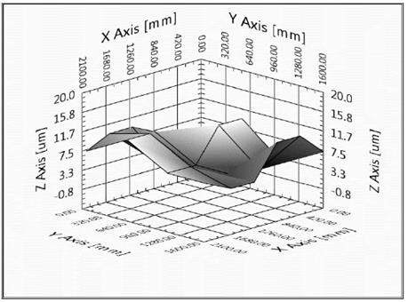
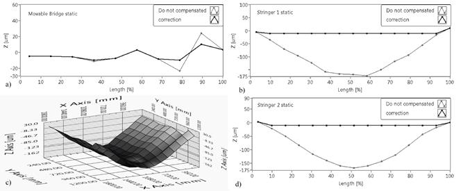
Figure 11 shows (c) the static deflections of each body including the initial misalignments (see Figure 10] and the corrections that the machine must perform at each point with a range of ±10µm . This Figure a, b and d, presents the static correction for (a) the movable bridge and for the stringer 1(b) and the stringer 2(d). The result of moving the axis of the machine following the path and at each point of analysis to evaluate the deviation; The maximum correction for the entire system is 171±10µm
Separately, it is obtained that for the movable bridge the maximum correction performed by the machine is 16±10µm , for the stringer 1, is 171±10µm and for the stringer 2, is 167±10µm. In Figure 11 c, the topology of the machine state is displayed in the workspace (2.16m 2 ) after execution [Figure 6]. Figures 11a, b and c are the views of the stringers and the movable bridge in two dimensions. Each figure shows the correction that the algorithm must have to compensate for the static error.
4.3 Dynamic compensation for continuous movement
Figure 12 shows the dynamic behavior of each sub-system of the machine. the movable bridge is a), the stringer 1 is b) and the stringer 2 is c), this figure illustrates the path already established at a constant velocity of 9m/min. The maximum correction of the system for that velocity is 27±10µm. Individually corrections due to misalignments, dynamic deflections for each are; for the movable bridge is 27±10µm, for the stringer 1 is 9.8±10µm and the stringer 2 is 27±10µm .
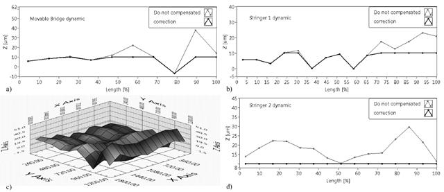
Figure 12 Dynamic deflection at each point, a) the movable bridge dynamic, b) the stinger 1, c) 3d static deflection and d) the stringer 2
Figure 12c, shows the dynamic topology generated by the machine.
4.4 Dynamic compensation for grinding process
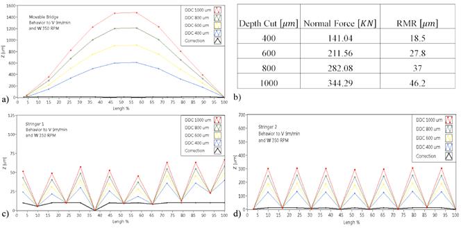
The structure of the machine in the slate grinding process was analyzed under the following operating parameters shown in Table 1. Firstly, Keeping forward speed and constant angular velocity, secondly, the attack angle of the tool was set at  degrees with respect to the horizontal, and thirdly, a width of feed on the X axis of
  of the diameter of the tool for the four cutting depth levels 400µm, 600µm, 800µm and 1000µm.
Figure 13 shows the shear depth deflection (SDD) in the machine structure during the depths of the cuts on a) the movable bridge and c) the stringer 1 and d) the stringer 2. In a similar way, Figure 13 b) presents the normal forces generated by the slate in the machine for each cut and the removal rate of material (RMR) in each step is obtained.
4.5 Control system error
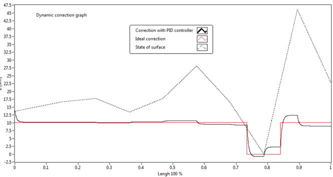
Figure 14 shows the correction tracking performed by the PID control of the machine on the bridge. The control installed on the machine delivers a maximum error of 3.6011µm during empty load travel at a forward speed of 9m/min.
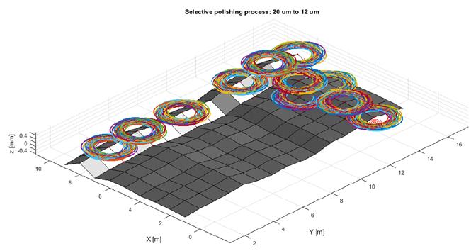
4.6 Selective polishing process
In Table 2, the parameters values used to develop the validation process are shown.
This process is accomplished to 12µm per meter of tolerance with a deviation ± 12µm. The zones where the polishing is performed are observed in Figure 15. The figure also shows the Archimedean trajectory that the polishing tool signed in each work area. The trajectory is based on the parameters established to reduce the flatness range of 12µm to 20µm. This process takes 2.402s per zone worked to remove an error of 8µm thickness. For the same case using the polishing process with linear path (see Figure 6], the work is completed in 4.819s per zone, hence the selective process takes 48.9% of the time that need the polishing process with linear path
5. Conclusions
Two complementary methods to improve precision in grinding tool machines are presented. A method to add precision in large machine tools with modular lightweight structures (APLM), which performs the compensation of the geometrics and dynamics errors using embedded intelligence. Secondly, an alternative polishing method called selective polishing (SP).
To achieve high precision in a lightweight machine in the grinding and polishing processes for petrous materials through the union of different mathematical models of the system behavior were developed. Firstly, it builds a process, secondly, it sets the measure in the order of microns, then it finds the low and high areas where you must make the corrections. Finally, information about future data position is inputted in a controller to makes the correction on time.
The tensioners must be used in lightweight machines to increase the stiffness of the structure, due the cutting forces in the materials produced in the structure produce a positive deformation (see Figure 13], which helps the algorithm to correct the error better in the machine.
Experimentally, it is observed that the vibration effects are maximized when there are great cracks in the surface or when the grain of the cutting tool between 80-120gr/in2 with a velocity of rotation of the spindle less to 150rpm. However, when it uses a cutting tool with a grain of 600gr/in2 with the same rotation velocity of the spindle, the vibration effect is minimized, and the grinded material is thinner. Therefore, lower grain cutting tools are used for grinding and others for polishing. As a result, the stringers with hollow pipe were built to inject a cement mixture and make the structure robust.
To achieve stability (see Figure 13] in the machine, the cutting forces are determined in relation to the translation speeds, rotation velocity, depths of cuts and angles of attack of the tool. Determining acceptable working vibration frequencies prevents the system from resonating when the control system is adjusted. In this case, the best behavior operation was achieved using a depth cut 10-400µm, and using an attack angle range of  .
.
For the final flatness work, if the polishing requirement is less than 67.8% of the piece area, the algorithm of selective polishing process generates more efficiency than the traditional polishing that covers the entire surface. The selective polishing process for petrous material reduces working hours and saving power consumption using embedded intelligence establishment of the higher areas and working intensely on them, until this within a tolerance of acceptance. The results using the selective polishing with an Archimedean spiral movement reduces in 48.9% the time of work machine in comparison with the polishing process with the rectangular path for the final path flatness.

