


 Inglês (pdf)
 Artigo em XML
 Referências do artigo
 Enviar este artigo por email
 Citado por SciELO
  Citado por Google
  Similares em
SciELO
Similares em
SciELO  Similares em Google
 Permalink
1. Introduction
Performing studies for determining environmental flows is part of a comprehensive management of basins and operation of rivers, reservoirs and aqueducts [1]. Environmental flows define the quantity, timing and quality of river flows needed to preserve freshwater ecosystems while assuring the continuity of human use. Insofar as they reduce water availability, and agricultural and industrial uses, Environmental Flow represents a constraint, but they also hold out new opportunities for development [2].
Environmental flows allow us to maintain the functionality and structure of aquatic systems and associated terrestrial systems in a sustainable way [3]. This contributes to keep rivers or transitional waters in good condition, and to achieve their ecological potential [4].
There are various methodologies for calculating environmental flows, such as hydrological methods, historical flow rates, hydraulic flow rates, habitat simulation and holistic methods [5]. These methods are the Natural Flow Regime, the Basic Flow Maintenance (QBM) and the Tessman method [6]. Some of these methods do not take the annual climate variability and effects of ENSO phenomena. For this study, the environmental flows were determined using the Range of Variability Approach RVA. The advantages of using RVA method is that it incorporates the hydrological and flow variability into environmental flow regime [7].
There are currently no estimations on a monthly and seasonal basis of environmental flows in the area. The Regional Autonomous Corporation estimates baseflow rates to determine the supply of water sources and manage resources, which are regularly updated. However, these values do not take seasonal variability into account. One of the existing studies for determining environmental flows in the area was performed by Universidad Nacional de Colombia [8]. Thus, the purpose of this research project is to create a calculation model to determine environmental flows taking into account variations of rainfall regimes from month to month and year to year.
In order to determine environmental flows for the water source, monthly rainfall registers of the most representative stations in the area, which are Olaya, Cotové, Juan García and Belmira [9]. Geomorphological parameters were also used in order to perform a hydrological balance of the basin that takes into account rainfall, aquifers, evaporation and infiltration. With this information, monthly mean flow rates of the water source were determined.
The study aims to stablish the environmental flows with the RVA method, using rainfall, infiltration and evaporation as main input data. This framework is especially useful in basins without flow rate registers.
2. Materials and methods
2.1 Collection of secondary information
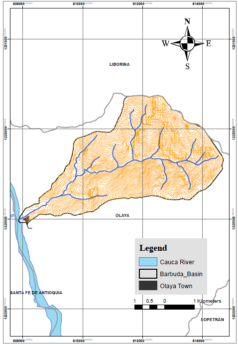
The basin of the Barbuda Stream is located in the Municipality of Olaya, Antioquia, in the North West of Colombia. It is the source of the water supply system in the municipality, and flows into the Cauca River.
The monthly rainfall data series of the stations Olaya, Juan García (Liborina), Cotové (Santa Fe de Antioquia) and Belmira were analyzed, [10] (IDEAM). The data series ranged from 1990 until 2014.
The area's topography and the cartographic plates from the Institute of Geography Agustín Codazzi [11] (IGAC) were used to demarcate the basin. Likewise, the drainage network and heights above sea level at which the basin is located were established. Figure 1 shows a panoramic image of the basin.
Based on the previous data, we obtained the geomorphological parameters of the water source. These will allow us to determine unknown variables of the site that have not been measured, such as evapotranspiration.
Previous hydrological studies contained in the Master Plan for the Water Supply and Sewage Systems [12], Wastewater Discharge Management and Sanitation Plan [13] and Program for the Efficient Use and Saving of Water of the Water Supply System [14] were checked. These studies have climatic and geomorphological data from the studied region. Apart from information about rainfall, aquifer contribution and soil infiltration rates, these studies include water source gauges. These data were used to describe the research area and to stablish basic parameters of the hydrological balance.
2.2 Collection of primary information: Fieldwork
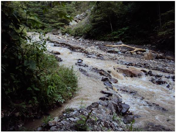
Gauges were performed in conjunction with the company in charge of the water supply system Regional de Occidente S.A. E.S.P. Speed-area methods were employed. These methods are based on the assessment of cross sections and flow rates per section through the use of floating devices. In addition, a rain gauge was placed in the water treatment plant operated by Regional de Occidente in order to assess rainfall in the area from January 2014 to October 2014. The activities mentioned were performed for the purpose of assessing the models. These models were calibrated to stablish correlations between parameters such as rainfall, evaporation and flow rate.
Selection of sampling sites
The gauges were performed at the water intake of the water supply system, located 1 km from the urban area.
The rain gauge system was placed in the Municipality of Olaya’s water treatment plant.
Gauging methodology and samples
The research followed the protocols of water monitoring established by [15] the Guidelines for Sanitation in Rural Municipalities and Small Communities [16].
IDEAM’s gauging methodologies recommend taking sections through which no more than 10% of the flow rate goes through because of the normal water source flow rate and the transverse length of the stream channel. To measure the total area, it was divided into five sections, facilitating the measurement of depth and width to approximate each section to selected geometric shapes. Then, the floating devices were thrown 2 m away in order to determine their speed by recording the time it took to cover the established distance. Figure 2 shows the place chosen for the activity.
Recording in digital format and data analysis
The information collected in the flow rate and rainfall gauges was recorded in formats established for performing the activity.
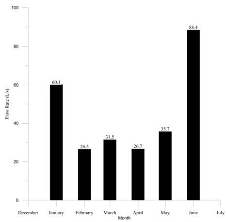
Regarding the flow rate gauges, the measures obtained with the monthly records [Figure 3] were compared.
In the case of rainfall, monthly rainfall accumulated amounts were measured. They were compared with rainfall data recorded by the Olaya station during the same month.
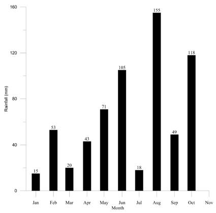
Figure 4 shows the rainfall recorded during the measuring activities in 2014.
Secondary information
As mentioned earlier, we collected rainfall data recorded by the stations nearby the basin between 1990 and 2014 [Figure 5]. They were used to determine monthly rainfall maximum and minimum, as well as the mean rainfall. Figure 6 shows the rainfall average recorded by the selected stations.
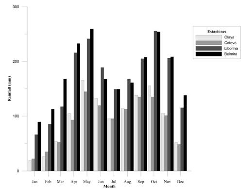
Figure 7 shows the maximum rainfall recorded by month in the Olaya station. It must be noted that it did not take place consecutively in a single year.
Figure 8 shows the minimum rainfall recorded by month. It must be noted that it did not take place consecutively in a single year.
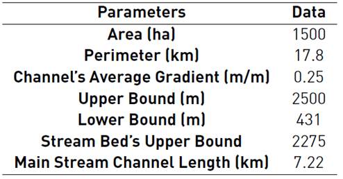
The basin morphometric parameters were consulted from Master Plan for the Water Supply and Sewage Systems Studies. Table 1 shows the main parameters of the studied basin.
2.3 Calculation models
In order to determine water source mean flow rates, and thus determine the environmental flows, a hydrological balance was performed. In it, we estimated run-off contributions and losses due to evaporation and infiltration based on rainfall and geomorphological parameters.
2.4 Determining basin shape and drainage parameters
Drainage density calculation
It is calculated by dividing the total length of the basin currents by the total area that contains them (Equation (1)]:
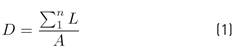
Where L is the length of the existing drainages, and A is the basin area in km2.
This rate allows us to have a better understanding of the complexity and development of the basin's drainage system. In general, a greater run-off density is a sign of a greater network structure or greater potential for erosion. Drainage density varies inversely with the basin's extension [18].
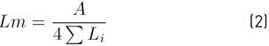
Mean flow length calculation
It is defined as the mean distance that water must cover in the basin to reach a channel [19]. It is estimated through the relation between the area and four times the length of all the basin's channels, or the inverse of four times the drainage density (Equation (2)].
Fluvial network hierarchical classification
The Horton method was used for the basin order's hierarchical classification [20]. This method numbers flow rates according to the tributaries that they have. Thus, the one that flows from the source and has no tributary is order 1, while the one that has two tributaries is order 2. If a channel has an order 1 tributary and an order 2 tributary, its order will be 3. The order of the channel increases one number at a time, so that even if a channel receives an order 2 and an order 3, its order would be 4. Each channel has a single order which will correspond with the highest order that it can have at the end of its course.
Mean basin height calculation
The mean height H is the average elevation with regard to the gauging station level at the basin mouth (Equation (3)] [21].
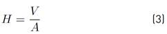
Where V is the volume between the curve and the axes. A is the basin area.
Height variation in a watershed has a direct impact on its temperature distribution, and therefore, on the existence of micro-climates and habitats typical of the prevailing conditions.
2.5 Use of rainfall data collected by the Olaya station
Rainfall is the variable with the greatest repercussion in hydrology because of its contribution to the total amount of water available in a hydrological system [22]. In mountainous areas, we must add the topographical influence to the stochastic nature of this variable in its spatial distribution [23].
As mentioned earlier, we used monthly rainfall records provided by the stations Olaya, Juan García, Cotové and Belmira because they are closest to the area studied. Based on these data, we calculated the mean rainfall using the Inverse-Square Law (ISL), whose Equation (4) is presented below [24].
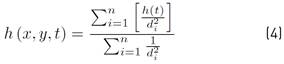
Where hi(t) is the height of the rain in the observatory i in the time interval t considered; di is the distance between the point considered (x, y) and the observatory i, and n is the number of observatories.
With the data provided by the stations mentioned above, we established the basin mean rainfall. The rainfall isohyets across the territory were also drawn. The Figure 9 shows the spatial mean rainfall distribution in the area studied.
The Figure 9 also shows the variation of rainfall distribution in the basin.
This was recorded in digital format, and the annual accumulated amounts were determined. Thus, it is possible to see the driest years and the periods with the most rainfall.
With these records, the mean rainfall was determined, as well as maxima and minima per month. Thus, it is possible to determine the driest and wettest months.
2.6 Evaporation and transpiration in the basin
Since there are no available data regarding basin evaporation and transpiration, these were determined through established equations. Below is the calculation of each established parameter to determine the variables.
Mean basin temperature calculation
Initially, the basin geomorphological data were used to calculate mean temperatures using the Equation (5) [25], which relates height above sea level to temperature variation. It is widely used in the country’s Andes region.
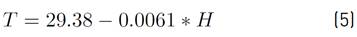
Where T is the mean temperature in ˚C, and H is the basin mean height in meters above sea level.
It is known that throughout the year, the monthly temperature average varies in the tropics according to the rainfall regime, cloud coverage, and to a lesser degree, solar radiation.
Therefore, monthly change percentages were estimated taking into account mean monthly temperature variation. These percentages were used to obtain monthly average temperatures for the basin studied.
Maximum and minimum temperatures were estimated using the averages established in the previous equation and the data recorded by the station Cotové. The values were assessed with a weighting process.
Basin potential evapotranspiration calculation
On the basis of the previous estimates, potential evapotranspiration was calculated using the [26] Equation (6) (1982).

In this equation, ETP is monthly potential evapotranspiration in mm, T is mean temperature expressed in °C, and Rs is incident solar radiation (mm/d).
Solar radiation plays a very important role in hydrological modeling in semi-arid environments, since it is a key variable for water circulation in the atmosphere.
In order to calculate incident solar radiation, the Equation (7) was used [27] SAMANI (2000).
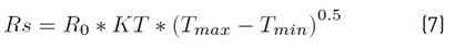
Where R0 is extraterrestrial radiation in mm/d; KT is an empirical coefficient that can be calculated on the basis of atmospheric pressure, but Hargreaves recommends a value of 0,162 for inland regions; Tmax is maximum ambient temperature, and Tmin is minimum ambient temperature.
Tables were used to determine R0, showing the monthly radiation mean values according to the geographic location in the area studied.
Monthly mean maximum and minimum temperatures were estimated on the basis of interpolation of data recorded by Cotové, located in Santa Fe de Antioquia.
Real evapotranspiration calculation
The Turc, and Coutagne Equation (8) were applied, and the results were used to determine an average.
The following expression is used to calculate the Turc equation [28] (1961).
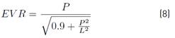
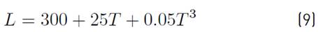
Where EVR is real evapotranspiration, P is annual rainfall, and L was calculated using the Equation (9):
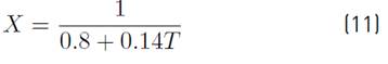
The Coutagne equation [29] (1954) is presented below (Equation (10)].

The equation data yield meters per year. The coefficient X is calculated as follows, (Equation (11)].
Determining evapotranspiration
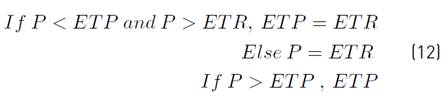
The evapotranspiration was obtained for each of the months and years of the assessment taking into account that when the rainfall is greater than the potential evapotranspiration, the latter becomes equal to real evaporation, (Equation (12)][30].
The ET’s obtained are the average ET's for all the Barbuda Stream's basin considering weather variation, which is related to height distribution.
2.7 determining flow rates
In order to determine the flow rate series, conceptual models have been used. The equations used for such models have a physical foundation, and they mean to simulate a basin's hydrological behavior through hydrological balance equations and equations of transfer among the diverse elements of the hydrological cycle [31].
The Stanford IV [32] and the Thornthwaite models are examples of this.
For this research project, the Thornthwaite model was used on the basis of a basin hydrological balance performed with the input flow due to rain, loss due to evaporation, and aquifer storage (considering soil properties). The baseflow was obtained with the surpluses. The model estimates that half of them become basin surface water. The equations used during this procedure are described.
Aquifer storage calculation
It is determined as a relation among rainfall (P), evapotranspiration (e) and storage capacity (W) in the soil as follows,[33] Thornthwaite and Mather (Equation (13)]:
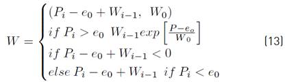
The Thornthwaite-Mather model [34] has had excellent results in Long Island (New York) [35] and Doñana Park in Spain [36] among others.
Calculation of surpluses in the basin
Surpluses relate rainfall to evaporation. There can be water surpluses only if rainfall is greater than evaporation, and if the soil is completely saturated (Equation (14)].

If the surpluses are lower than 0, the value will be 0.
Run-off calculation
Aquifer contributions, that is, a month’s run-off in particular, is obtained by adding the following month’s surpluses according to the series developed by Thornthwaite (1957), adjusted through coefficients, in which the effect of vegetation is included [37] Alley (1984) for several models, (Equation (15)].
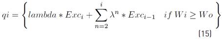
According to soil storage calculations, the model adjusts to the T model proposed by Alley (1984), in which a coefficient λ of 0.75 for small basins is established. Thornthwaite suggested using a λ of 0.5. Therefore, it is selected considering that the Barbuda Stream is classified as such because its area is less than 20 km2.
The results are calculated using the basin area and relevant conversion factors in order to obtain the run-off flow rate series to be used in subsequent analyses.
2.8 Environmental flow estimation
The flow rate series determined with the hydrological balance explained previously were used to estimate the environmental flows. The RVA methodology [38], Simplified models [39] and the concepts developed by Aguilar and Polo (2014) [40] were also employed. The procedure is presented below.
The RVA uses 33 hydrologic parameters to evaluate potential hydrologic alterations. Seventeen hydrologic parameters focus on the magnitude, duration, timing, and frequency of extreme events and geomorphology; the other sixteen parameters measure the central tendency of either the magnitude or rate of change of water conditions [41].
The methodology has been used for the determination of ecological flows in different research works, such as those conducted in more than 30 basins located in the United States of America (USA) and Canada [42], as well as in South Africa [43], Australia [44], and Spain [45].
Flow rate distribution function
A relation between each flow rate and the total number of determined flow rates recorded + 1 was calculated using the Equation (16).
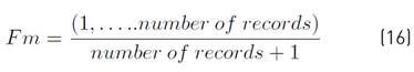
The distribution function was expressed as the relation between the parameter Fm and the determined flow rates, from the lowest to the highest. The figure shows the distribution function obtained for the flow rate series.
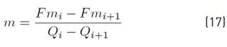
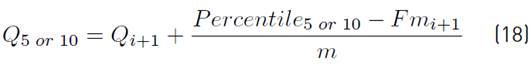
Estimation of percentiles 5 and 10
Percentiles 5 and 10 indicate the flow rate value, below which are 5% and 10% of the records in the group of total observations [46]. As the data group was ordered from lowest to highest, the fraction is for lower flow rates [47].
Each percentile was determined on a monthly basis by performing an interpolation of the relevant curve segments with a programming language developed on MATLAB, which translates as finite differences into the following expression (Equations (17) and (18)]:
Determining environmental flows for the barbuda stream
The percentiles determined were used for environmental flows per month. Percentile 5 is the environmental flow that must be kept in dry periods, that is, the years in which an abnormal rainfall decrease takes place. Percentile 10 refers to wet periods, or years in which rainfall is above average.
In order to have water supply values, these can be compared with monthly flow rate averages in the source.
3. Results and discussion
3.1 Secondary information
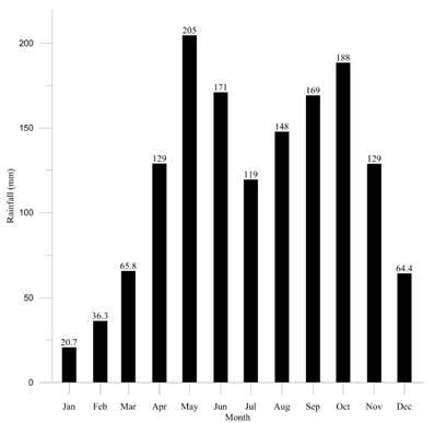
In Figure 5, a bimodal trend is observed in the rainfall [48]. It shows two periods of special intensity in April-June and September-November. The greatest rainfall accumulation takes place in May. Dry periods comprise the months December-March and July-August. The least rainfall takes place in January and February.
During the research period, we noted important “El Niño” climate phenomena for 1992-1994, 1997 and 2002 years, and significant “La Niña” climate phenomena for the 1995-1996, 1998-2001 and 2010 [49]. The minimum and maximum rainfalls values were recorded during Boy and Girl phenomena periods [50], respectively [Figures 6 and 7].
3.2 Basin shape and drainage parameters
Table 2 shows the shape and drainage results determined for the Barbuda Stream basin using the equations mentioned in the previous section.
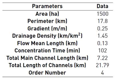
According to the parameters determined, we can establish that the basin studied has a very small area: less than 20 km2 [51]. It has an elongated shape because of its perimeter.
According to the results obtained, the basin has low drainage density, since it is between 0.5 and 1.5.
Based on the mean flow length parameter, we can determine that the distance covered by a drop of water from any place in the basin is short, which can be associated with high gradients in the area.
The basin mean gradient shows us that it is located in very uneven ground with steep slopes. Therefore, water flow can cause very strong flash floods.
According to the basin order, determined with the Horton index, it is classified as a meso-scale basin, since the value obtained is between 4 and 6.
3.3 Rainfall as measured by the stations
After using the ISL method to calculate the spatial mean rainfall, rainfall isohyets of the region determined by the stations were created, as shown in Figure 9.
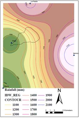
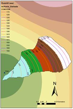
It was determined that the annual mean rainfall in the basin is 1398.9 mm. The basin is influenced mainly by the areas close to the Cauca River, which are characterized as a tropical dry forest life zone. The rainfall regime in these zones ranges between 1000 mm and 2000 mm per year [52]. Figure 10 shows the drawing of rainfall isohyets within the basin, for which ArcGIS 10 was used.
The mean rainfall results are influenced by much wetter areas located at the top of the basin, close to the stations Belmira and Juan García. Therefore, the rainfall average recorded by the stations is slightly superior to those obtained in the areas alongside the Cauca River. However, the result tends to be similar to the one established for that region [53].
The annual average rainfall distribution, calculated on a monthly basis with ISL is shown in Figure 11.
3.4 Basin evapotranspiration
Extraterrestrial solar radiation
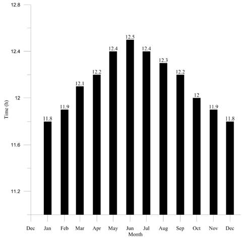
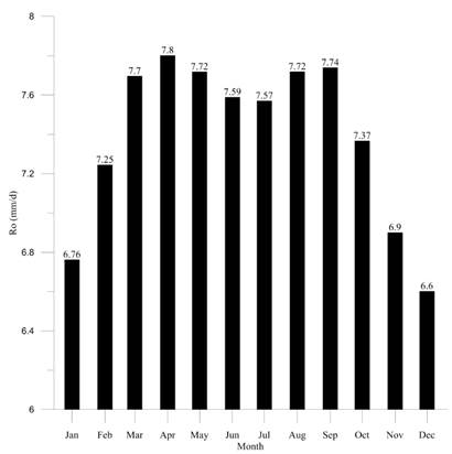
Initially, the data related to the number of hours of solar irradiation and radiation for every month of the year were used to determine the extraterrestrial radiation perceived in the basin area by applying relevant conversion factors to express it in mm/d. Data are shown in Figure 12.
Temperature distribution
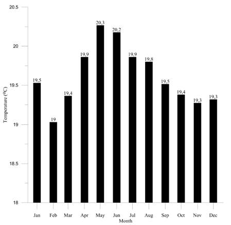
The determination of basin mean temperature took into account the distribution of areas. According to the altitudinal zone, it is 19.6 °C. The value obtained was used to calculate the temperature distribution month by month, as shown in Figure 13.
Incident solar radiation
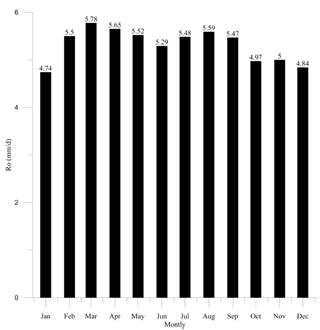
By using the expression mentioned above, maximum and minimum temperature values obtained for the basin, incident solar radiation and other coefficients were incorporated. Thus, the incident radiation results, referenced in Figure 14, were obtained.
Potential evapotranspiration
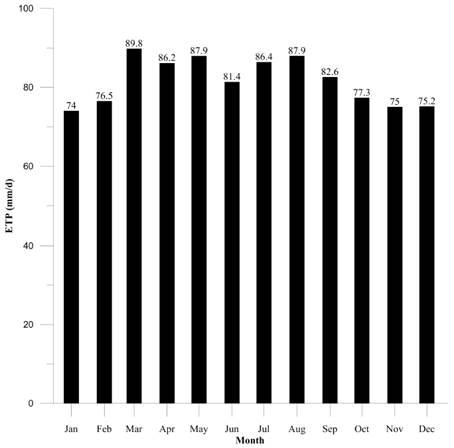
The Hargreaves equation with the incident solar radiation results and temperature distribution was used to determine the potential evapotranspiration values for each month of the year. The results are shown in Figure 15.
Real evapotranspiration
Based on the rainfall series obtained with ISL and the temperature distribution in the basin, the real evapotranspiration was determined using the Turc, and Coutagne equations. Temperature data were used to determine parameters associated with the equations.
An annual value of 1167.68 for L was obtained with the Turc equation, and of 0.282 for X with the Coutagne equation.
Annual ETR results are presented in Table 3.
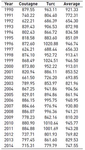
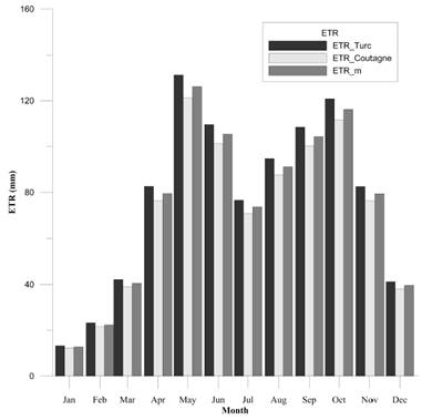
Figure 16 shows the real evapotranspiration results obtained month by month with each equation and their average.
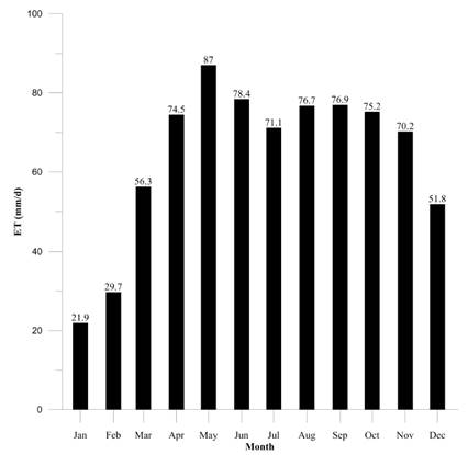
In order to determine ETR results month by month, the averages of the equations applied were used. This was also applied to the ETP results. Thus, the ET results for each month of the years for which there are rainfall records were obtained.
Based on the relations between real and potential evapotranspiration and rainfall, we obtained the final ET results to estimate the hydrological balance. Figure 17 shows the average results estimated on the basis of final ET results, which were used for the hydrological balance.
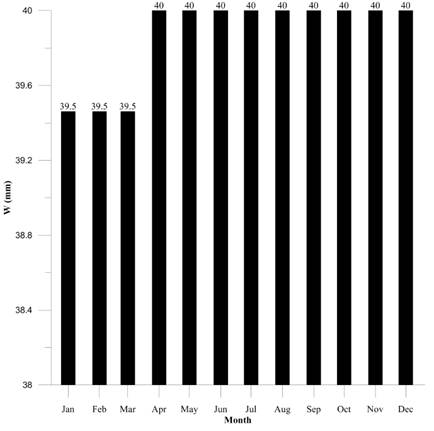
3.5 Aquifer storage
The relations between rainfall and evaporation were used to obtain average results for the years studied [Figure 18].
During the first months of the year, the amount of water stored in the soil decreases. This is also true in August, which is not surprising, due to the decrease of rain and increase of evapotranspiration during that time.
Surpluses
The surpluses were determined on the basis of the relations rainfall/evaporation/aquifer storage capacity established in the previous sections. Thus, monthly results were obtained for each year analyzed. The averages are presented in Figure 19.
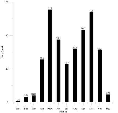
It is observed that minima are reached in January, February and March. Even though rainfall increases during these months, the rain will mostly infiltrate the soil because of the lack of rainfall at the beginning of the year, which reduces moisture storage. Then the soil reaches its saturation level, and surpluses gradually increase.
3.6 Monthly average flow rates
The water source average flow rates were determined using the series established for calculating aquifer run-off, which takes into account surpluses of the previous month, as well as previous accumulated amounts. The results were obtained for every month of every year studied. With these values, a flow rate average of 24 years was determined. Besides, the maxima and minima of the series were established. The above can be seen in Figure 20.
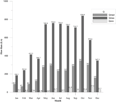
It is generally observed that the flow rates obtained tend to be higher during the months with more surpluses and rainfall, especially in September and October.
3.7 Environmental flows
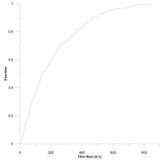
With the flow rates obtained, the data distribution function was determined. It is shown in Figure 21.
After applying the methodology described, we obtained the following series of minimum flow rates associated with percentiles 5 and 10, which are for extremely dry or wet periods. Table 4 shows the results.
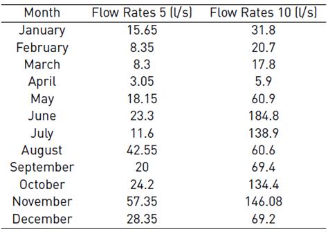
Minimum environmental flows occur during the periods of lower aquifer storage rates, that is, in February, March and April. These coincide with the periods mentioned before, since there are droughts during December, January and February, so accumulation of water in the basin decreases. This period lasts until April because, despite the rain, the soil has just begun to recharge[54]. Therefore, most of the water infiltrates the soil, and there is little surplus contribution.
The RVA approach enabled the analysis of the hydrological changes of the River. The results [Table 4] show that hydrologic changes of mean monthly flow in the dry (January, February, March and August) and wet periods (April, May, October and November) are more obvious than other months in the transition periods. The annual climate variability was stablished. The flow rates in extremely wet periods are two to three times higher than dry periods.
During baseflow periods, the basin can reach values of up to 3.05 l/s. This is a sign that there may be little surface water supply and shortages for the various uses that water is given along the channel, which is an issue because this is the water source of the municipality and many surrounding villages. Therefore, hydrological planning is suggested on the basis of this study’s results in order to make the most of the resource during times of drought.
According to CORANTIOQUIA, the Barbuda river had an available flow rate of 102,3 L/s for water supply. According to the findings, the available flow rate value exceeds the environmental flows stablish in dry periods. However, it is putting at risk the water supply.
4. Conclusions
The mean flow rates obtained with the method implemented match those gauged at the source for each of the months and years evaluated. Therefore, it has been proved that the model created is a useful tool to calculate flow rate series when there is little rainfall data.
Rainfall distribution in the area is mainly affected by the dry regimes that take place near the valley of the Cauca River. However, rainfall increases gradually as height increases in the mountain. Therefore, a mean rainfall that exceeded that of more representative basin life zones was obtained.
Flow rates maxima and minima are monthly averages, therefore, the peaks may be higher or lower for shorter time scales.
According to the geomorphological parameters assessed and the observations that took place, the basin can be classified as a ravine. The criteria for this classification are based on the steep gradients, little storage capacity in the soil and scattered vegetation cover, typical of life zones classified as tropical dry forest.
The flow rate series obtained show great variations between the flow rates recorded during wet and dry periods. This is in tune with a basin classified as a ravine.
The environmental flows obtained with this methodology, with regard to years with a drought trend, ranged between 3.05 l/s during drier months and 57.35 l/s during rainy months. With regard to years with more rain, environmental flows between 5.90 l/s during drier months and 184.8 l/s during wetter months were obtained. The results determined match those expected for a basin such as the one evaluated, and they have been verified against previous records.
The model developed in this study is perfectly applicable to similar basins. The only primary information required will be rainfall data, geomorphological parameters and mean temperatures. In order to obtain more accurate results, detailed rainfall series, such as those recorded on a daily basis, must be used. Thus, maximum and minimum flow rates will be determined within a clearer time scale.
We used the environmental flows obtained to determine that the basin flow rates may decrease greatly, even to levels of total drought. This will significantly affect the population that benefits from the water source. This might cause a health emergency in the region or prevent agricultural activities that represent the livelihood of many families.

