


 English (pdf)
 Article in xml format
 Article references
 Send this article by e-mail
 Cited by SciELO
  Cited by Google
  Similars in
SciELO
Similars in
SciELO  Similars in Google
 Permalink
1. Introduction
Currently, production systems (PSs), such as secondary cooling systems, present new organizational structures as an effective response to challenges, such as production focused on demand and high variability in product requirements [1, 2]. In this context, a PS with a centralized structure has evolved towards a distributed structure, where the specialized core, which manages the available resources for the production of goods in a traditional structure, is divided into several subsystems that are interconnected by a communication system. This enables information to be concurrently processed on multiple modules to share resources [3]. Thus, improvements are made based on particular system variations in each module within the system; that is, the characteristic of modularity gives the system a structural flexibility that facilitates a response to changes and enables the system to be scaled by adding specialized modules in certain productive processes.
However, a correct definition of distributed structure demands several challenges to be overcome, such as the availability of specialized resources, integration methods for the modules, coordination of treatment information centres, reliability, security, and increased dynamic of systems [4]. Thus, this study addressed the issue of an adequate specification of a distributed PS using a formal tool, such as: Coloured Petri Nets (CPN). In these cases, the distributed PS is considered a discrete event system (DES), where a DES is a dynamic system that evolves according to the asynchronous occurrence of certain discrete changes, which are referred to as events [5].
A CPN is a mathematical formalism and graphical tool that enables the formal description of systems, whose dynamics are characterized by the concurrence, synchronization, mutual exclusion and conflicts, which are characteristics of a distributed PS [6, 7]. Several studies that employ this approach demonstrate its effectiveness [7-11]. The advantage offered by the models developed with CPN compared to other types of Petri nets is the possibility of interpreting the values of the variables (temperature, presure, etc.) at each change of state during the process. Moreover, the use of this formal tool for system modelling improves its understanding, identifies its main features, facilitates improvement strategies with a discrete approach, among others [12].
This paper proposes the use of this modelling tool for the specification of a distributed system: the secondary cooling system Chiller, which is located in the E33 building of the School of Mechanical Engineering at the Universidad del Valle in Cali, Colombia.
The article is divided into six sections distributed as follows: section 1 presents an introduction to the article context, section 2 provides a brief description of the system, its requirements, use cases, and architecture. A description of how the cooling system was modelled is described in section 3. Next, section 4 presents the system CPN model and then its validation is shown in section 5. Finally, conclusions are presented in section 6.
2. System description
2.1 System components
The refrigeration laboratory of the School of Mechanical Engineering at the Universidad del Valle in Cali, Colombia, has a cooling system, Chiller, which employs a steam compression cycle with a nominal load of 20 TR (tons of refrigeration). This system is employed in research, comfort applications and academic practices.
Its operation is based on the pumping of icy water to the spaces to be cooled by using terminal units (for example, fan-coil and thermal floors) for the heat transfer between the air of the spaces and the frozen water. This secondary cooling system operates at night or early in the morning and produces the amount of ice (thermal reservoir) that is required to supply a cooling load at peak times. The cooling system consists of three cycles: evacuation (3), cooling (2), and load (1). Figure 1 shows the devices and sensors distribution for the temperature, pressure, flow and level measurement and recording. The sensors are represented by a circle with a letter, which represents the measurement variable, and a number, which indicates the sensor number.
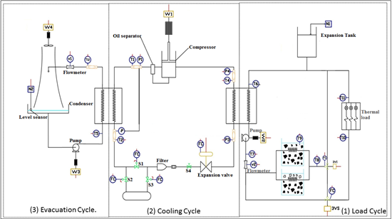
Figure 1 Scheme with the sensor locations and system variables. (1) Load cycle, (2) cooling cycle, and (3) evacuation cycle
In the load cycle (1), the heat is extracted from the room to be cooled using a mixture of water and glycol, which flows through a piping circuit. The cooling cycle (2) is a vapour compression refrigeration cycle, which employs refrigerant R22 to extract the absorbed heat in the load cycle. The evacuation cycle (3) evacuates the heat transmitted from the condenser to the water that circulates. In Figure 2, the refrigeration equipment is shown; its components are detailed in Table 1.
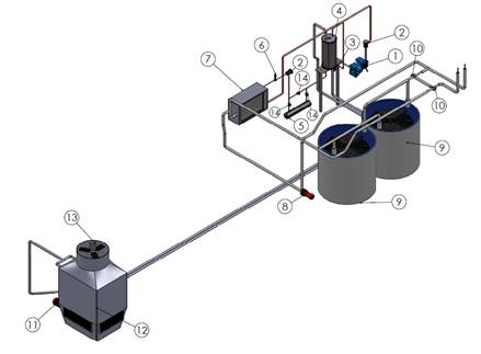
Figure 2 Chiller (School of Mechanical Engineering, Universidad del Valle, Cali, Colombia). (1) Compressor. (2) Dryer filter. (3) Oil separator. (4) Condenser. (5) Accumulator. (6) Expansion valve. (7) Evaporator. (8) Pump, 3 hp. (9) Ice Banks. (10) Three-way valves
2.2 System requirements
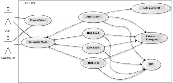
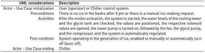
The system considers two main operation modes: manual and automatic. Manual mode activities are managed by an operator, whereas the automatic mode poses a self-regulated operation with minimal human intervention. Auto mode comprises four sub-modes: Low Charge Mode, Medium Charge Mode, High Charge Mode, and Night Mode. The low, medium and high modes are configured according to the cooling load demanded by the area to be conditioned. These three modes primarily vary by how they fill the cooling load. The charge in the night mode is a function of the ice banks production. Due to space limitations, a special description in night mode is provided. A UML diagram of the use cases was constructed; refer to Figure 3 and its description in Figure 3 and Table 2.
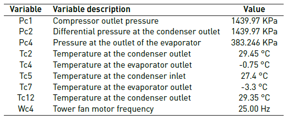
The night mode requires that the system produce 5 TR during ten hours by freezing two 2000 L water tanks. At this point, the values of the variables that dominate the dynamics of this operation mode are estimated. These variables are associated with the pressure, temperature and flow measured by the sensors, operation frequency, and water levels in the cooling tower and glycol tank.
The night mode operates with fixed parameters in the load cycle, compression and evacuation until the required glycol temperature is attained at the evaporator outlet (T7). Then, the glycol mass flow in the load cycle is modified to compensate variations and maintain a stable temperature (T7). In the vapour compression cycle, the compressor inlet pressure (P4) and the coolant temperature at the evaporator outlet (T4) are obtained by manipulating the mass flow of refrigerant through the evaporator. Additionally, the pressure (P2) and temperature (T2) are regulated at the condenser outlet by manipulating the mass flow through the condenser with the compressor. The evacuation cycle is operated by modifying the water mass flow to control the water temperature at the condenser outlet (T12) and modifying the cooling tower fan operating frequency (W4). The water cooling rate is varied at the condenser inlet (T5) to maintain stable heat extraction variations. A summary of the theoretical values for the system variables are shown in Table 3.
2.3 Distributed architecture of the cooling system
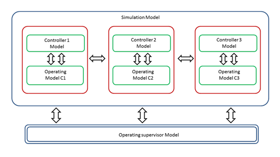
The control system architecture established a distributed process management in three autonomous control elements (controllers) according to the chiller cycles. In addition, it was considered to be a supervisor to coordinate the autonomous controllers; the proposed structure is shown in Figure 4.
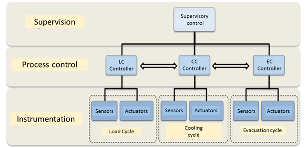
A hierarchical structure was proposed, in which the supervision level is composed by the supervisory control, here the operational interface tasks are carried out with the operator and the control supervision system; At the level of process control, the control and resource management routines are performed, which is composed of the controllers of each system, and the last, the level of instrumentation is conformed with the elements that interact with the process and record their information. This study did not use specific communication protocols.
3. Secondary cooling system modelling
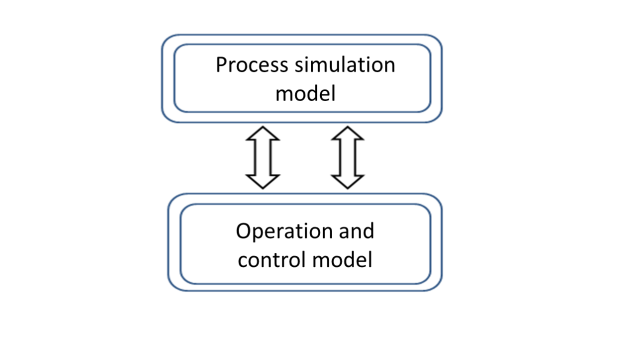
To address the Secondary Cooling System modelling, a Bottom-Up approach was employed [13]. A global system representation is constructed, and via successive refinements, it defines the components and their interactions and establishes the system behaviour. The model consists of a model that enables the process simulation and an operation and control model, as shown in Figure 5.
3.1 Process simulation model
The simulation and validation model employed the following procedure:
First, all system components that influenced the process dynamics, i.e., actuators, sensors and other devices, were listed.
Second, each system device was modelled using Coloured Petri nets (CPNs), a detailed description of this tool is provided in [14]. To enable these models in order to emulate the behaviours of real systems, thermodynamics and mechanics relations, which govern the respective phenomena in the devices, are employed.
Third, following a bottom-up approach, once the devices’ models were obtained, the cycles modelling that structured the general model were performed. Thus, the models that belong to each cycle are interconnected and linked using the relations that govern the system behaviour. The initial approximation that is used to join different elements was established according to the real plant distribution.
Finally, the three cycles’ models were interconnected by their relationships to establish a general simulation model, which emulates the system behaviour and its variables during Chiller operation.
3.2 Operation and control model
The operation and control model employed the following procedure:
Once the control architecture was defined in section 4, a control model scheme was obtained, as shown in Figure 6, which consists of a supervisor model and three control models (green schemes), with one model for each cycle’s system (red schemes). The arrows between the different blocks indicate how the elements interact through the interface, which are represented by the boundary of each block.
The control system approach was performed for each cycle system as each cycle has a different control program. The operation model is divided into three main elements, which coincide with the operating states of each cycle: Start (“Start”), Run (“Operating”) and Shutdown (“Off”). Each of these operating states has different action sequences depending on the mode of operation. These sequences are modelled for each cycle: start sequence, which corresponds to the adjustment of the valves, verification of the levels and the start, followed by each cycle operation, i.e., their control methodologies. The shutdown sequence is modelled; all information is based on the Chiller operation manual.
A supervisory control model, which coordinated and synchronized different operation modes, was proposed. This model was proposed using the same structure as the control cycle models: Start, Run and Shutdown.
4. Model description
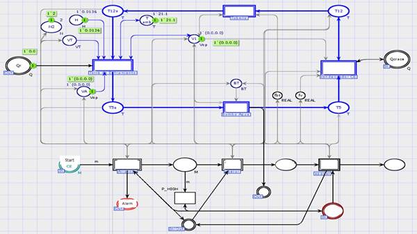
The Chiller CPN model is shown in Figure 7. Three sets of elements are distinguished: circles or ovals, rectangles and arcs (arrows). The circles represent places; the rectangles, transitions, and arrows represent the flow information and trigger conditions.
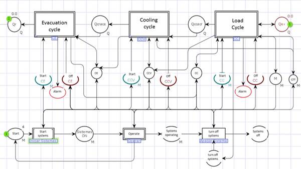
The model is structured as shown in Figure 6, where the upper rectangles to double lines represent the cycle models. The model at the bottom, which is bounded by the Start (“Start”) and System Off (“Systems off”) places, represents the supervisory control model.
Additional arcs and places, which are arranged between the two models enclosed in the dotted line in Figure 6, represent the communication elements between the models, that is, they represent the order flow and recognitions between the supervisor and individual controllers. Places within this zone represent on (“Start”) and off (“off”) commands, which are exchanged between the supervisor and the individual controllers. The "cc", "ccv" and "ce" locations emulate the check signals sent by the individual controllers to the supervisor to indicate a task completion. The arcs that come off and arrive at the components of the supervisor's operating model represent the flows of information that are exchanged between the supervisory control and the different controllers of each cycle. The information flow also occurs between the controllers and the resources they manage, i.e., the sensors and actuators of each cycle.
Double-line transitions are a high-level model abstraction: Load, Cooling and Evacuation cycles. A detailed representation of these transitions integrates both the simulation and the operation models of each cycle. Considering the space limitations, only the Evacuation cycle model and some of its components are presented.
4.1 Evacuation cycle model
To perform this simulation model, the dynamics of its respective components were represented, as shown inTable 1. The pump model is shown in Figure 8.
Initially, both the states that it can achieve and the events that encourage the evolution of these states were raised. For example, the running pump state can be altered by the occurrence of the pump off event.
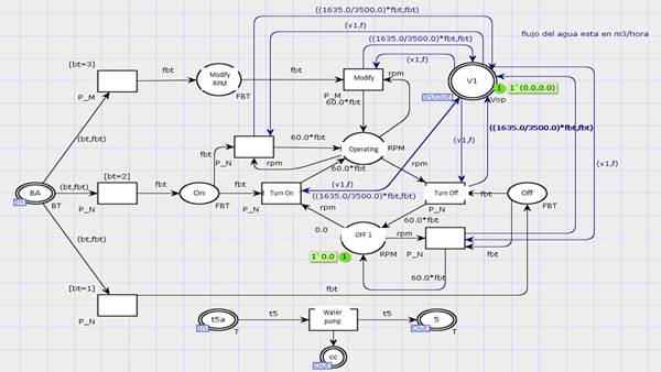
The pump model is presented in Figure 8; this model represents the pump behaviour and its speed variator. It is composed of transitions and places and double-line places, where the blue labels "in", "out" or "in/out", represent ports that interact with elements outside of the pump, such as the location "V1", which represents the flow recorded by the flow sensor in this cycle. The "BA" location represents a load cycle controller order (C-CC), after which the order is classified as an order to modify the pump operating frequency, whose representation is in a place with the same name, or as an order to turn on the pump-place "On"-or a command to turn off the pump-"Off" place. In the middle, the running ("Operating") and off ("OFF") locations represent the pump state. In this case, when it is off, it registers 0.0 rpm, which is the value in green, and when the pump does not operate, the flow through the registered cycle by sensor V1 is 0.0 m3/h and frequency 0 Hz. The modify ("Modify"), shut down (“Turn off”) and power ("Turn On") transitions represent the action execution denoted by its name. Additional transitions to the centre, without a name, emulate other action executions; for example, when a power command is received ("On") and when the pump is operating (operating state) to continue system operation.
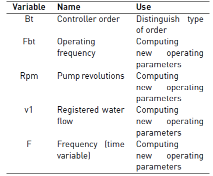
Above the arcs, a series of inscriptions that represent the relations that govern pump operation are observed. In this case, the equations compute the flow delivered by the pump as a function of the frequency operation. The variables in this model are clarified in Table 4.
After obtaining the models of the components involved in the evacuation cycle, the integration of these elements was performed to construct the simulation model of the Evacuation cycle shown in Figure 9.
Evacuation Cycle model has three sets of elements. The elements in black represent the start, operation and shutdown events (operation model and cycle control). The blue elements represent the components involved in the evacuation cycle, pump, cooling tower and fan. The grey elements, the arcs, represent the information flow between the components and the controller. The Evacuation cycle operation model has arcs to exit places (ports); these elements represent the information exchange between the autonomous controllers and supervisory controller.
The "T5", "T5a", "T12" and "T12a" locations were arranged to emulate the fluid state to the devices’ outputs and inputs. In addition, the "T5" and "T12" locations symbolize the temperature sensors that are located along the flow line of the evacuation cycle. The "Qcrace" and "Qr" places emulate the thermal load that is transferred from the refrigerant to the water and the load rejected to the environment. The "fv" and "fbt" locations emulate the temporary controller variables and are employed to synchronize the processes. "N2" emulates the water level sensor status in the tower; "BT" represents the existence of commands to modify the pump operation; and "H" and "T amb" are the humidity sensors and dry bulb temperature of the environment, respectively.
5. Model validation
5.1 Model validation procedure
Model validation was performed by process simulations to verify that each model element and the integration system components correctly operate; some test scenarios were proposed.
During the simulations, an operation mode and the required thermal load for each scenario were initially established. Subsequently, an algorithm that generated a required thermal load change was established to generate a disturbance, emulate a step input, and observe the process behaviour before the control model action. The respective simulation was executed for each test scenario, and the information recorded by the sensors was compiled. The information was collected using observers at certain points of the model, with which data, such as temperature and flow, were extracted; this information was tabulated in worksheets and graphs were elaborated to analyse the process behaviour and interpret the worksheets and graphs.
The networks were reviewed to ensure that no locks, infinite repetitions that consume resources, untransferred places and transitions, and networks that do not fit the actual system are reviewed.
5.2 Simulation scenarios
The selective simulation scenarios for validation included the operating scenarios that introduced the system to critical situations. These situations are observed in mode changes. The results for the Night Mode are presented in this section.
In the Night Mode simulation, the system behaviour during ice generation was emulated. As initial conditions, the banks water temperature was already 0.3 °C because we wanted to analyse the moment at which they begin to freeze the water deposits without assuming that the simulation would have the required time. The initial glycol temperature was -3 °C. The variables observed during this scenario were the evaporator temperature (T7), the glycol pump operation frequency and the ice banks temperature (T9); these elements are located in the Load Cycle.
5.3 Results - Night mode operation
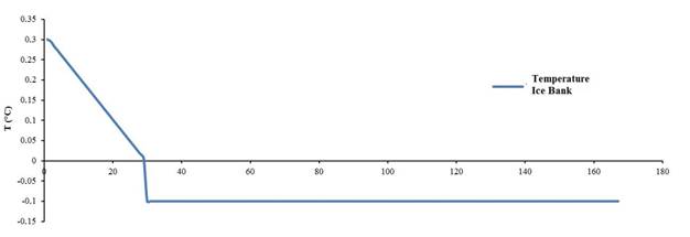
Figure 10 presents the simulation results during the cooling and subsequent freezing phases in the ice bank. Temperature measurements were taken during the operation (ten hours), where the temperature stabilization is observed after four hours and nine minutes until reaching a temperature of -0.1 degrees Celsius.
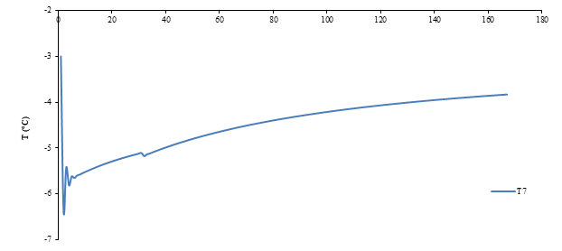
Since the ice banks temperature is directly related to the temperature of the evaporators, the results obtained from the simulation of glycol temperature at evaporator outlet are shown in Figure 11, starting with the temperature graph at the enclosure entrance. The graph shows the behaviour of this element during the same time of simulation performed for the ice banks temperature. A decrease in the glycol temperature at the evaporate outlet was initially observed; the subsequent increase in the glycol temperature occurred when the control action attempted to stabilize the temperature at -3 °C. The initial decrease occurs when the glycol temperature at the exit of the ice tanks is 0 °C, and the temperature decreases further when passing through the evaporator. At this point, the control action modifies the pump operating frequency to increase the glycol flow rate and obtain the desired glycol temperature. The small variation in the glycol temperature, between shots 20 and 40, is attributed to the fact that the water temperature in the tanks reaches 0 °C at this point and begins the process of isothermal freezing.
In the same way the glycol pump operation frequency variation is shown during the same operating time (simulation) in Figure 12. It is observed that to maintain the glycol temperature at the evaporator outlet, the control action must increase the glycol flow rate in the cycle.

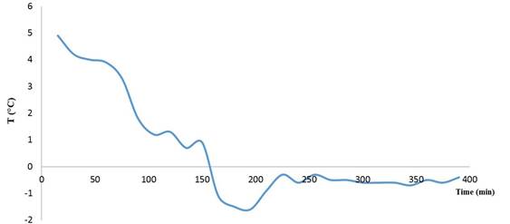
Based on the results obtained in the simulation of the model made in CPN tools, the real system was configured to verify its behaviour, as shown in Figure 13. In spite of presenting considerable variations with the simulated model, a similar behaviour is observed in the shape of the obtained curve. These appreciable variations may be due to the fact that the equipment had been in disuse for several years without maintenance. This project made it possible to reuse this team and verify the importance of the use of formal models, for instance CPN tools, to ensure that both the operation and performance of the system are adequate.
6. Conclusions
Currently, industrial or residential applications of a secondary cooling system are varied. Considering the dynamics of these markets and the demand of an agile response to the variation of the contexts, the distributed structures in this type of applications has been stimulated. In order to correctly specify and use the associated technical and human resources, the use of formal tools is recommended. In this sense, this paper presented a systematic approach that enabled the characterization of the secondary cooling system located in the Mechanical Engineering School at the Universidad del Valle, and proposed a distributed architecture. In this manner, semiformal and formal modelling tools, such as: UML and Coloured Petri Nets, respectively, were integrated to characterize the system. Initially, operational requirements were identified from the perspective of the needs of the system’s users using UML diagrams. Those models were detailed up to distributed control structure specification using Coloured Petri Nets. The design was outlined in three operative levels: monitoring, process and instrumentation. The experimental results allow us to validate the approach presented to obtain the model which will allow future improvements of the proposed structure according to new demands.

