


 English (pdf)
 Article in xml format
 Article references
 Send this article by e-mail
 Cited by SciELO
  Cited by Google
  Similars in
SciELO
Similars in
SciELO  Similars in Google
 Permalink
1. Introduction
Surface water quality is one of the fields of natural resource management that has recently been addressed in the national scenario as a response to the gaps identified in environmental regulations, and the permanently increasing tension on water resources exploitation. Within this field, public policy strategies that include the monitoring of surface water sources have been developed. In Colombia, water quality models have been implemented in different case studies [1-3] to simulate temperature dynamics, dissolved oxygen (DO), biochemical oxygen demand (BOD) and total suspended solids (TSS). Within the territory, there is a significant progress in the implementation of water quality models, consisting of complex structures due to the number of processes they represent; however, heavy metals models are still at a very early implementation stage. In this regard, representing the complex number of chemical and physical reactions that are established in these constituents make the available models costly or difficult to access, because of the amount of information required for the implementation in our environment [3-5].
Certainly, heavy metals naturally occur in streams in highly variable concentrations since they are part of the geological composition of the soil; but human activities, especially those taking advantage of natural resources (such as mining, exploration of hydrocarbons and different industries) have favored their presence in water bodies in higher concentrations, which might be dangerous to health, given the toxicity of these elements. Indeed, there is a potential impact on surface waters, due to heavy metals concentration because of the activities mentioned above; this is why water resource managers need tools that allow them to define regulatory strategies based on criteria, with the aim to improve decisions regarding Water Resource Management.
Likewise, the heavy metals modeling takes on an enhanced significance, due to the need to predict the behavior of metals in water, especially in our environment where information is limited, being necessary to establish tools that allow more effective results under these scenarios to be obtained, and support management processes of environmental control entities, including the planning stage.
Therefore, this article proposes a strategy to predict the behavior of heavy metals, including a view from the reach scale to the basin scale, which allows the implementation of the method to different instruments of planning and management of the water resource.
2. Theoretical framework and state of the art: transport and water quality models
Water quality in streams is influenced by the transport and reaction processes, which include chemical, biological and physical conversions generated over time and space. Transport processes refer to advection and dispersion processes, while reaction processes refer to the transformation of water quality determinants, such as BOD, COD (Chemical Oxygen Demand), TKN (Total Kjeldahl Nitrogen), DO, among others.
Research conducted in recent decades on the behavior of solutes in lotic systems, has improved the development from the transport model to the development of the ADZ (Aggregated Dead Zone) model (6, 7), which allows adequately modeling the storage effect of one or more dead zones (stagnant zones). The model, represented by Equation (1), uses the concept of two zones, a first region where the solute is transported during a period by pure advection processes and a second well-stirred region in which the solute is dispersed before being released at the end of the stream reach [8].
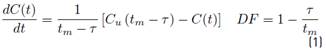
where t represents time [T], Cu(tm - τ) [ML−3] is the upstream concentration entering the reach, C(t) [ML−3] is the output concentration at the downstream boundary [ML−3], tm [T] is the mean travel time and τ [T] is the lag time or first arrival time (travel time) and DF [dimensionless] is the dispersive fraction. The travel time tm and the lag time τ are easily measured in the field using curves by performing tracer experiments.
Furthermore, Equation 1 adequately describes the tributary inflow containing conservative substances; however, for non-conservative substances, [9] developed an improved version of the QUASAR (Quality Simulation Along River Systems) water quality model, which, in addition to the advective and dispersive processes represented by the ADZ simulation scheme, incorporates sinks or mass sources from the substance modeled by first-order reactions.
Equation (2) represents the ADZ -QUASAR model (the ADZ model, and the Quality Simulation Along River Systems, QUASAR), where k [T-1], corresponds to the reaction constant related to the modeled substance, thus integrating both the dynamics of solute transport and the transformation of constituents:

where Ʃ inputs and Ʃ outputs refer to the possible inputs and outputs of the modeled substance in the reach.
3. Materials and methods
3.1 Description of the study area
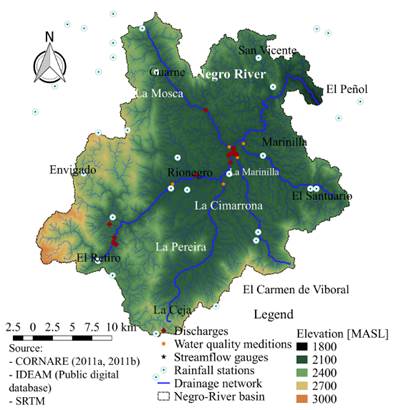
The study area is located in the department of Antioquia, Colombia, within the Negro river basin, which has an area of 5924.83 Km2, made up of the municipalities of Guarne, San Vicente de Ferrer, Rionegro, El Carmen de Viboral, La Ceja, Marinilla, El Peñol and Envigado. The Negro river headwater is located to the south of the region, on the eastern side of Las Palmas mountain range, in Cerro Pantanillo (municipality of El Retiro) at 3000 m.a.s.l. By the municipality of El Peñol, it is called the Nare river, and receives Pantanillo, La Pereira, La Mosca, La Marinilla, La Cimarrona and La Compañía streams [10].
The basin morphological and hydro climatological conditions make it a water-producing system, with average annual precipitation of 2200mm and an average temperature of 18°C. The basin supplies the area of the San Nicolás Valley; the reservoirs of La Fé and Piedras Blancas supply drinking water for the northeast and the southern sector of Medellín and its metropolitan area, moreover, the basin also supplies the Peñol-Guatapé Reservoir System, which generates the third part of the energy of the country. Currently, the basin faces complex environmental and social issues, due to the settlement of large industries on the corridor of the Medellin-Bogotá highway; in addition, the largest populated centers of the East region are concentrated in this area, a condition that puts a strong pressure on the land and its uses, and directly affects the water quality [10].
Figure 1 shows the location of the Negro river basin and the evidence available regarded as secondary data, which is described later.
3.2 Secondary information
The digital elevation model (DEM) was available with a resolution of one arc-second, interpreted by NASA from the products of the SRTM (Shuttle Radar Topography Mission, available in http://gdex.cr.usgs.gov/). Hydrological analyses included information on the vector drainage network, scale 1/25000, developed by Agustín Codazzi Geographical Institute (IGAC-by its name in Spanish) and available in the Geographic Information System for Planning and the Territorial Organization (SIGOT. http://sigotn.igac.gov.co/sigotn/framespagina.aspx).
Daily record precipitation was used, based on data for 70 rain stations, which are part of the network of stations of the Institute of Hydrology, Meteorology and Environmental Studies (IDEAM by its name in Spanish).
Temperature is essential to calculate and determine the kinetic reactions for water quality indicators along a stream [11]. In this work, valuable advances by [12] are considered, who found from statistical regression analysis that in Colombia the average annual temperature and the elevation above the mean sea level are strongly correlated [12]. For the Colombian Andean region (the area in which the hydrological analyses are carried out), the expression found by these authors is described in Equation (3).

where T is the average annual temperature in degrees Celsius and h is the elevation above the mean sea level in meters.
In order to constitute the baseline of water quality, information was taken from CORNARE, the head of environmental regulation in the study area that has been developing projects and measurement campaigns in different locations close to the area and established the water quality guidelines for the different streams. CORNARE investigated the water quality of the principal streams and its relation to human activities in the region [13]. This paper collects secondary information of [13] to establish the baseline of the Negro river in the modeling exercise. CORNARE water quality information includes water quality sampling in discharges and streams in different periods during the years 2003-2008; the database has information for dissolved oxygen, electrical conductivity, pH, total suspended solids, BOD, TKN and several heavy metals, among which, copper, chromium, and nickel are to a greater extent in the basin and the discharges. For this reason, they are selected as the heavy metals to be analyzed in the present study.
3.3 Hydraulic characterization and dispersion mechanisms
The water quality model implementation under lack of information requires establishing metrics for determining the most important variables so as to define general characteristics from empirical models.
Based on the morphological classification system (descriptive level) proposed by [14], the reach selection or morphologically homogeneous reaches shall be determined, establishing for each reach or section the full bankwidth, WB , the full bank height, HB , and the reach slope, S. If possible, the dominant bed morphology should be identified, characterizing its shapes and granulometry.
From the initial proposals developed by [15], the concept of hydraulic geometry is still used as an instrument for the estimation of morphological characteristics of streams, including relationships between variables such as width (W), average speed (U), and the average depth (H) with the flow rate as shown in Equation (4):

where ai and bi are constant and depend on the morphological and hydraulic characteristics and the subscripts w, h and u refer to the width, depth, and average speed, respectively.
According to the conceptual representation of the ADZ model, properly describing the dispersion mechanisms in a stream reach is equivalent to defining the values of the parameters tm, τ and DF for a given flow condition [16]. The experiment with tracers is widely used to experimentally identify the travel time and the dispersive fraction representative of a stream reach, factors directly related to the mechanisms of solute transport.
Although the effects that a discharge has on a body of water depend on the magnitude of the load discharged, it is very important to determine the self-purification capacity of the streams via a natural process. The latter is closely related to the hydraulic properties of the system and, likewise, includes the biological or chemical processes that lead to the degradation of the specific substance being analyzed.
In Colombia, several approaches have been developed with the aim to empirically estimate these parameters. [16] found close relationships between travel times and flow. Similarly, [9] and [17] present strategies for calculating tm and ( through the MDLC-ADZ (including the Multilinear Discrete Lag Cascade of channel routing, MDLC, and the Aggregated Dead Zone model, ADZ), simulation scheme that allows developing the flows and solutes transport in a stream reach in a coupled way. [18] analyzed the behavior of the variability of the dispersive fraction in mountain rivers and found that it has high variability unlike the plain rivers, finding that its magnitude can be established in DF=0.272±0.015.
Due to the lack of hydraulic information in the Negro river system to carry out the water quality simulation, the contributions of [9, 16-18] for the characterization of solute transport mechanisms in the drainage network were adopted in this work following the methodology proposed by [6] and [18].
Considering that there is not detailed hydraulic information and that this is needed to simulate sedimentation, re-aeration, and resuspension processes, a hydraulic section was calculated using the secondary data provided by IDEAM in the cross-sectional profiles at each recording station. The IDEAM information for these sections contains data on the cross-sectional profile, flow rate, velocity and depths associated with each gauging in the profile.
3.4 Model implementation
The water quality simulation was carried out in a stable state, which means that the characteristics of the system do not change with time and that the discharges involved are active at all times during the simulation window.
Modeling heavy metals is a task that requires considering a significant number of interactions. For instance, reactions with different constituents of the suspension matrix, the dissolved matrix, and the sediment bed, provide an intricate series of possible reactions that turn the task into a complex modeling exercise. Figure 2 shows the conceptual model for heavy metals behavior.
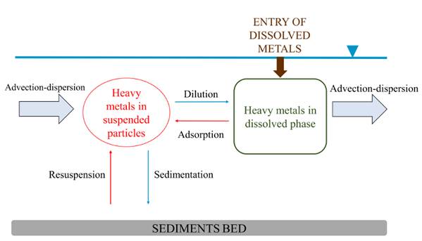
Heavy metals usually react with different constituents of the dissolved and suspended matrix in various forms. For this reason, it is expensive to obtain all the information required for a complete description of the reactions of heavy metals in water. Therefore, some authors [4, 5] have tried to reduce the degrees of freedom in numerical modeling exercises in order to solve the complexity of the reactions. However, this work seeks to evaluate the predictive capacity of a water quality model based on the parameters that can have a significant impact on the heavy metal’s behavior and that are widely evaluated in sampling campaigns, in order to obtain a flexible modeling tool that can be applied in an environment with lack of information.
The present methodology does not develop the modeling of heavy metals considering the characterization of the subspecies of all the components, because this type of modeling requires a robust volume of data and characterization. For this reason, the different species of chromium, copper, and nickel are not included; however, these reactions are considered for the determination of the level of significance of variables such as suspended solids, pH and dissolved oxygen, in each of the stages of the proposed methodology.
Temperature, electrical conductivity, pH, and dissolved oxygen directly affect the dissolution capacity of heavy metals, in addition to the kinetics of transport and transformation reactions [5, 20], moreover, TSS affect the adsorption capacity of the suspended material [4, 5]. These constituents are sampled extensively and are part of the regulatory requirements in the Colombian territory [21]. Considering the limitations and complexity of heavy metals modeling, this research paper adopts the equation where the general scheme of simulation for heavy metals in the ADZ-QUASAR simulation structure is presented (Equation (5)]. This approach is consistent with previous modeling strategies of wide application in Colombia [3, 22].

where Kmetal [T-1] is the degradation constant of each specific metal and is obtained from the Equation (6), H [L] represents the average depth of the characteristic section of the reach, Vt [LT-1] represents the average speed of the section and Fpsed [dimensionless] is the suspended fraction of each base metal calculated from the partition coefficient of the sediment layer proposed in [23], according to Equation (7).
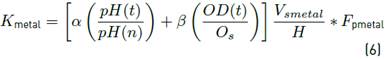
where pH(t) represents the pH value and pH(n) the neutral pH value, DO(t) [ML-3] is the dissolved oxygen value and Os [ML-3] is the saturation dissolved oxygen value, and Vsmetal is the sedimentation rate of each constituent specie (chromium, copper, and nickel for this case).
where [TSS] is the concentration of total suspended solids at each point [ML-3] and Kdsus is the partition coefficient of suspended matter for each metal [L3M-1]. The partition coefficients can be extracted from [23], which has specific ranges for each metal analyzed in this study. Fp [dimensionless] is the present particulate or suspended fraction and is calculated as shown in Equation (7). Parameters ( [dimensionless] and β [dimensionless] are model adjustment parameters and vary depending on the representativeness of pH and dissolved oxygen for each specie in particular. The degradation constant of each metal ( Kmetal ) is corrected according to the temperature of the water in each point using the following equation (Equation (8)]:

where K(ºC) [T-1] represents the correction of the degradation rate of the metal due to the water temperature and ( is the Arrhenius constant, in this case taken as 1.047, and T(t) is the water temperature in degrees Celsius at time [°C].
Vsmetal [LT-1] is the sedimentation rate of each constituent specie (chromium, copper, and nickel for this case) and is calculated from the ratio between the particle diameter and specific gravity as proposed by [24] (Equation (9)].
where Gmetal [dimensionless] corresponds to the specific gravity of the metal, ( [LT-1] to the kinematic viscosity, g is the acceleration of gravity (9.8067 m/s2) [LT-2] and d (mm) is the diameter [L] of the sediment particle.
3.5 Calibration and uncertainty analysis
Calibration
The main objective of the calibration is “to test” the global behavior of the model and its response to variations in physical and numerical parameters. These variations must be made within a real range [25, 26].
Given a description of the system to be modeled, the values of some variables can be predicted at the output of the system. This problem of predicting results is called a modeling problem, a simulation problem or a direct problem. The inverse problem consists of using measurements on some variables to infer the values of the parameters that characterize the system [27].
The process of using measurements on some variables of a system to infer the values of the parameters that characterize such a system is called calibration [25, 26]. It is a process of adjustment of parameters that intend to reproduce the behavior of the results obtained in the observed environment with the simulated results. Because in the dynamic water quality models there are multiple responses (at least one for each modeled pollutant), that are related to the parameters of the model in a non-linear way, it is difficult to develop the adjustment manually and the explicit linear-regression type solutions are not possible, so more sophisticated iterative techniques for the estimation of parameters are required.
In order to ensure the correct performance of water quality models, it is necessary to establish a sequence of elements related to the dynamics of the behavior of the substances to be simulated, which correspond to:
Hydrological component: the implementation of the model is proposed under medium-flow conditions, taking into account the average conditions of the concentrations (and loads) of discharges and water quality analysis at the control points.
Hydraulic component: The hydraulic characterization of the selected modeling section will be made using a regionalization technique that considers the main components affecting the behavior of the substances to be simulated, this regionalization will be carried out from the available information of cross sections with the information that IDEAM has in the study area. This exercise will be carried out for the flow width, the velocity of the stream and the bottom depth of the bed, as presented in Equation 4.
Transport mechanisms: The mechanisms of transport, dispersion, and diffusion of the different pollutants, as well as the determination of travel times, are adopted from the calculated empirical relationships referenced in [16], where the correlation of these mechanisms with the hydraulic geometry of the section can be observed.
Estimation of calibration parameters and model uncertainty
The GLUE (Generalized Likelihood Uncertainty Estimation) methodology is used [28], which rejects the idea of a single "optimal" solution, explaining the best fit between model results and observed data, trying to obtain a group of combinations (inputs, structures, parameter sets, errors) that are consistent in behavior with observations (not error-free) [27]. It is implemented by means of Monte Carlo simulations [29], to find a series of groups of parameters that describe the observations with different levels of approach. The GLUE methodology allows the uncertainty of the parameters in the simulation implementation [30] to be quantified based on the performance analysis of the parameters and the evaluation of their goodness of fit. For the current implementation, the analysis of different objective functions (multiobjective) that allow evaluating the correct performance of the random combinations of parameters is proposed. Different functions are analyzed to evaluate the confidence of the results obtained from the model with the values registered within the stream stations (goodness-of-fit), by comparing both secondary and primary information taken in the field. The performance functions applied to the evaluation of the results were the Nash-Sutcliffe efficiency coefficient (NSE) [31], the Relative Percentage Bias (PBIAS) [32] and the Coefficient of determination [27].
3.6 Description of the application exercise
Two modeling exercises were carried out; in the first one the calibration of the model parameters is performed with secondary information [13]. In the second exercise, the validation is carried out with information taken from the field.
First modeling exercise
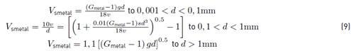
The selection of the analysis reach for the first exercise was made based on the availability of information. A simulation length of approximately 32.18 km was determined, establishing stations in the river as border conditions, in order to initiate the values of the constituents from the estimated records. Figure 3 shows the selected simulation section for the preliminary modeling exercise.
The sampling campaigns used for the modeling exercise were based on secondary data [13] (taken in isolation in each sampling station without linking the travel time between them). This modeling exercise considers the following features:
The simulation was carried out in a permanent flow state, taking into account as input flow, the average daily flow in the period of recording of physicochemical information available in [13].
The first measurement station located in the section is regarded as a boundary condition for the simulation section. In the same way, the most important tributaries, with continuous monitoring of water quality, have as the boundary condition the first station from upstream to downstream with water quality data.
The monitoring stations with water quality data found in the Negro river (and the tributaries) will be considered as control points. The records available in these stations will help to corroborate the model's performance through the fit measurements described in section.
The results of the model will be evaluated, within a multiobjective framework, with the average value obtained in the records in the data period available in [13]. Additionally, the probability distribution function will be analyzed, in order to ensure that the performance meets the expected values for each of the control points.
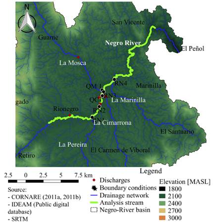
Figure 3 Selection of the first section for the preliminary simulation exercise with secondary data, taken from IDEAM, SRTM databases and [13]
Second modeling exercise
In order to carry out the validation of the model, a field campaign was conducted in the analysis section of the Negro river on June 23, 2016, to collect water quality information in six (6) points, distributed in approximately 7.5 kilometers of section comprising the sector with the most significant impact associated with the discharge of 10 pollutants into the stream. The places were strategically located in order to facilitate the sampling and collection of cumulative impacts on the tributaries to the Negro river. Figure 4 shows the location of the reach and the water quality sampling points, and each of the water quality and quantity monitoring sites, both for the Negro river and for the influential tributaries in the section of interest, according to the following conditions:
The simulation will be carried out under a permanent flow condition, having as the input flow the discharge measured during the campaign.
The boundary condition in the modeling section on the Negro river is established at the first monitoring station. This station is located downstream of the main discharges on the river that might interfere in the modeling activity.
The largest amount of discharges, especially industrial, occurs on the main tributaries that converge into the Negro river. This individual characterization of the discharges is beyond the scope of this study, thus the physicochemical analysis of each of these tributaries is carried out in the nearest accessible point to the confluence, along with the interpretation of the IDEAM limnimetric station level, so as to establish the flow at the time of characterization. This is developed in order that, given the difficulty of quantifying individual discharges, these are added to the stream before joining the main section.
The measuring stations on the Negro river are used as control points that allow determining the goodness of fit of the model.
The parameters ( and ( found for each of the heavy metals studied in the first modeling exercise remain unchanged in this exercise, in order to analyze the effective representativeness of these in the dynamics of the system.
Figure 4 Location of the validation section of the heavy metals model and selection of water quality monitoring points. Information taken from IDEAM, SRTM databases and [13]
Stations on the Negro river
In Figure 4, the points referring to the Negro river and its tributaries are presented along with the validation section of the model. Station RN1, on the Negro river, is used as a boundary condition for the model. With reference to RN1, the travel times of the water body were calculated, trying to collect the samples downstream the section from the same upstream reference site. RN2 station, which is located upstream of the confluence with La Cimarrona stream is highly affected by the municipal wastewater, in addition to discharges from the food industry, among others. In the RN3 station, which is located upstream of the confluence with La Mosca stream, it was possible to observe the continuous discharge of industrial wastewater towards the river. At this point, the river collects the waters of La Cimarrona stream which contains discharges from industrial use. Finally, station RN4 acts as the closing point for the section of interest.
The stations QC1 and QM1 were located in La Cimarrona and La Mosca streams, respectively. These stations are located in accessible sites close to the confluence with the Negro river and give information about the accumulated impacts before unloading on the Negro river, regarding discharges by the textile, pharmaceutical, and food industries, among others.
Flow results in station RN1
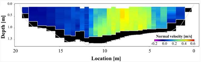
The equipment used to measure flow parameters in the cross-sectional area of the RN1 station was a river surveyor M9 which is an Acoustic Doppler Current Profiler (ADCP). Figure 5 presents the gauge selected at the RN1 station, where the bathymetry of the wet area section estimated from the ADCP path can be observed. The estimated flow rate for the section at the RN1 station was 3.8 m3/s; which represents the flow rate from which the loads for the boundary and the following conditions were calculated.
4. Application of the model and results
A simulation based on secondary information collected from [13] is carried out. After the implementation of the proposed heavy metals model using secondary information, a validation exercise is proposed with information collected in the field for the verification of the methodology. The procedure of the aforementioned application exercise is described below.
4.1 Hydraulic characteristics of the study area
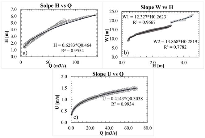
Figure 6a shows the relation between flow and mean depth and Figure 6b shows the relation between bank width and mean depth. In Figure 6b, it can be seen, at approximately 3.2 m deep, a shift in the relation between depth and bank width, allowing to define potential characteristics for each depth section. Finally, Figure 6c shows the relation between flow rate and average flow velocity.
It is noteworthy to mention that these characteristics are fundamental, since the processes of sedimentation, advective transport, aeration, and resuspension, are defined from the hydraulics of the environment. Regionalized relationships allow describing these characteristics in sections and segments of the study area where information is not sufficient. For this reason, the use of these relationships makes it possible to carry out simulations on regional scales, where information at the stream scale may be scarce.
However, these relationships are closely related to the area of study. Therefore, it is necessary to determine this behavior in the study area whenever a water quality model needs to be implemented. Additionally, in case of having a more detailed hydraulic model, this can be used to determine the components that depend on hydraulics.
4.2 Modeling results of the first exercise - calibration
Below are the results of the exercise carried out with secondary information, from which the initial calibration of the model was carried out, in addition to the sensitivity and uncertainty analysis.
Sensitivity and uncertainty analyses
The sensitivity analysis is focused on determining the representativeness of important changes in the input variables (pH, temperature, dissolved oxygen, and total suspended solids) of the heavy metal model and its response at the end of the simulations. Thus, different simulations were performed for each of the heavy metals analyzed, with extreme values defined individually for each of the variables. The model results do not exhibit sensitivity for temperature variations and total suspended solids, whereas the variations of pH and dissolved oxygen show a greater sensitivity and noticeable changes are evident, especially for chromium and nickel; although in the case of copper, the model is more sensitive to changes in dissolved oxygen and secondly to variations in total suspended solids, so the adhesion mechanisms may be important in the model. However, it is clear that the model is more sensitive to variations in dissolved oxygen, so a good simulation strategy and an adequate collection of field information for this variable suggests a better performance in the results of the model (detailed results of the sensitivity analysis are presented in [19] and are also shown in Figure 7].
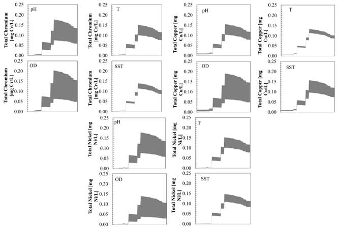
Figure 7 Sensitivity analysis for total chromium, copper, and nickel associated to variation of pH, temperature, dissolved oxygen and total suspended solids
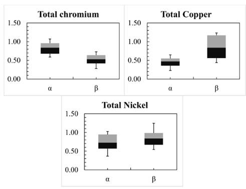
Additionally, taking into account that the parameters of the model represent a series of combinations that allow an adequate performance in the different random model runs, an uncertainty analysis for each of the heavy metals being an object of study, with different combinations of the parameters of the heavy metals model was developed. After 10000 simulations, it was possible to conclude that there are few variations, so it can be said that the model has little associated uncertainty [19]. Figure 8 shows the results of these 10000 simulations and the uncertainty of these exercises.
Temperature, pH, TSS, DO, BOD 5 and TKN modeling
Figure 9 shows the results for temperature, pH, TSS and dissolved oxygen. The BOD and Nitrogen as TKN model results are also shown, which strongly influence the behavior of dissolved oxygen (because they are directly related to oxygen consumption and, therefore, to its dynamics in streams behavior).
The lines shown in blue in Figure 9d correspond to dissolved oxygen saturation, which is taken as reference. The black boxes represent the mean value of the parameters at different points (with their characteristic error bars); this differentiation of the monitoring and verification points with error bars was done because the temporality of the secondary data does not allow defining conditions of transient simulation, since sampling was carried out in different monitoring scenarios and in different periods.
The results observed in the graphs presented in Figure 9 show a good adjustment between model results and field measurements. This is corroborated with the results presented in Table 1 which represent an adjustment proposed within the work presented by [19] and [33]. The results depicted in Table 1 are related to the sensitivity analysis, for which the pH and dissolved oxygen are the most important variables when evaluating the response of the simulations.
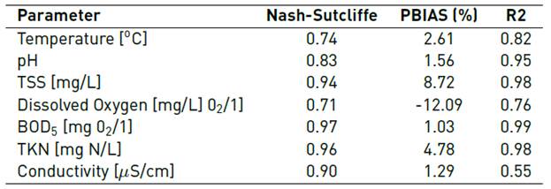
Table 1 Result of the performance estimators for the support variables of the model in the preliminary exercise
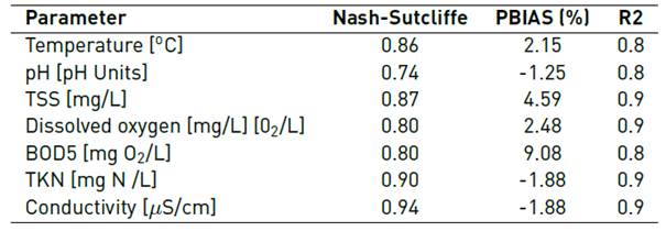
The pH modeling, despite having an estimate in the Nash-Sutcliffe coefficient less adjusted than the other parameters, is in an adequate range and the value estimated in the bias ensures that the results are reliable, being an important entry for the heavy metal model.
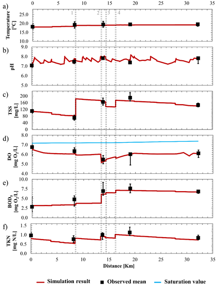
Figure 9 Results of support variables for the preliminary exercise. a) temperature, b) pH, c) total suspended solids d) dissolved oxygen, e) BOD5, f) TKN. The double vertical lines represent the tributaries entering the Negro river: 1- Pereira stream, 2- La Cimarrona stream, 3- La Mosca stream and 4- La Marinilla stream
Heavy metals (copper, chromium, and nickel)
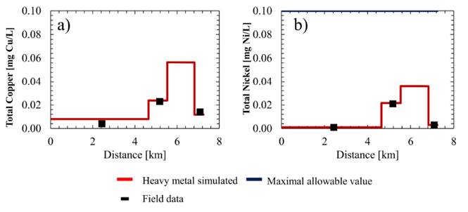
Figure 10 shows the simulation for the three heavy metals analyzed in the present study (chromium, copper, and nickel).
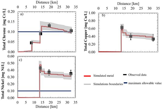
Figure 10 Heavy metal simulation result for the preliminary exercise. a) total chromium, b) copper, c) nickel
The blue lines shown in Figure 10a and Figure 10c, correspond to the minimum limit required in discharges according to Resolution 631 of 2015 of the Ministry of Environment and Sustainable Development of Colombia (by which the parameters and the maximum permissible limit values in the punctual discharges to surface water bodies and public sewage systems are established) [21]. Finally, the two dotted gray lines represent the maximum and minimum values obtained from 10,000 Monte Carlo simulations made from the variation of the characteristic diameter of the particles, the density of the metal and the partition coefficient (see Equations (5) to (9)].
Figure 10a presents the modeling of total chromium. The chromium simulation includes modeling of the hexavalent and trivalent species in a separate way because each of these has a characteristic behavior in the streams and different kinetics dynamics [23, 34]. However, since the records by [13] present information of total chromium, the result of this modeling is presented as the sum of the hexavalent and trivalent chromium species in Figure 9a. Figure 10b and Figure 10c present the modeling for copper and nickel, respectively.
Results shown in Figure 10 refer to an exercise of 10000 simulations, where the gray region includes all the possible results of simulations and the red line represents the better adjusted simulation to the obtained values. The overestimation observed in the copper values and the underestimation of the total chromium and nickel values can not only be associated to the adjustment of the model, but also to the quality of the data used to calibrate the model. That is, the sampling exercise did not follow a strategy of travel times and the data corresponds to a set of samples taken at different times between the years 2003-2008. Although the model simulation shows overestimation and underestimation, it is observed that the red line (simulated metal) is located along the width of the boxplot (observed data), for the three heavy metals considered.
4.3 Modeling results of the second exercise - validation
Results for the modeling exercise referred to the field sampling, defined for the validation exercise of the methodology are presented in the following sections.
Laboratory Results
Table 2 shows the laboratory results obtained for the six (6) monitoring stations presented in Figure 4.
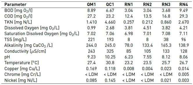
<LDM lower than the detection limit.
The sampling campaign for the validation exercise shows for chrome and nickel heavy metal results below the detection limit in several stations. In the case of total chromium, five stations show values below the detection limit, so it is not possible to validate the results of the methodology for this metal.
Station RN1 represents the boundary condition of the analysis section. Nickel values in this station are below the detection limit, for this reason, the boundary condition in the analysis section for this metal is estimated as the value of the detection limit (0.001mgNi/L), being the most unfavorable condition in water quality assessment, these results are corroborated later with the simulation downstream and the analysis of the objective function in the R1, RN2, RN3 sites which suggests that the initial nickel values are close to the one suggested.
The results of dissolved oxygen, BOD5, COD and TKN presented in Table 2 show a significant degree of contamination, which lowers dissolved oxygen to values close to zero for tributary streams of the Negro river (La Mosca and Cimarrona Streams). These streams are the most affected by discharges of industrial effluents.
Similarly, the pH values of La Cimarrona stream (pH = 10.25), indicate in some way the possibility of contamination of industrial origin with the presence of heavy metals, because the processes of elimination of these require high pH that favor the formation of precipitate salts and might be eliminated by sedimentation.
These high pH levels favor higher metal removal rates nearby the discharge and decrease the removal capacity as it goes along the path and the pH tends to stabilize. However, this sedimentation capacity of heavy metals is reduced by the absence of dissolved oxygen, which for the different compounds derived from heavy metals tends to favor the solubility of these in low concentrations [20].
Temperature, pH, TSS, DO, BOD 5 and TKN modeling
Based on the water quality results presented in Table 2, the values obtained in RN1 were established as a boundary condition, and values obtained in stations QC1 and QM1 were set as the quality values of the tributaries. For this reason, the stations RN2, RN3, and RN4 provide the reference values for the model. The results of the evaluation of this performance appear in Table 3 and the results of the full modeling are shown in Figure 11. In the same way that for the preliminary exercise with secondary data, it can be seen that the adjustment of the model is properly fitting the observed data.
Table 3 Results of the performance estimators for the support variables of the model in the validation exercise
The dissolved oxygen results presented in Figure 11d, have a lower precision possibly because this parameter was not estimated with all the possible nutrients reactions. However, the dissolved oxygen values obtained in the model were in a range of good estimation. The parameters of water quality, in general, present approximations close to the observed values. The results in the modeling of BOD5, TKN, and TSS, report modeling values in the estimators, such as the Nash-Sutcliffe coefficient and coefficient of determination, very close to one and biases relatively close to zero, which indicates that the valuation method is reliable [32,33].
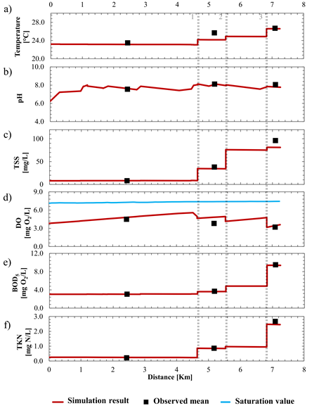
Figure 11 Results of support variables for the validation exercise. a) temperature, b) pH, c) total suspended solids, d) dissolved oxygen, e) BOD5, f) TKN. Double vertical lines represent the tributaries feeding into the Negro river: 1-. La Cimarrona stream, 2- La Mosca stream, 3- La Marinilla stream
Results for the selected heavy metals
Figure 12 shows the copper and nickel simulation. The red line was modeled with optimal values of the parameters ( and (, used in the preliminary exercise, in order to validate the results found in the first approach.
5. Conclusions and recommendations
It is clear that the available water-quality data is subject to different hydrological and hydraulic scenarios, making it difficult for being used transparently in calibration and validation (control) scenarios. In order to overcome these difficulties, the historical values of water quality associated with the average flow were considered and the simulations were developed from a permanent flow scenario. However, this condition in some cases may lead to underestimating and, in other cases, to overestimating the actual contamination. The inclusion of a water quality model such as the ADZ-QUASAR model implies a decrease in the volume of information needed for modeling, and its simplicity in programming is used for the construction of a distributed model that allows the solution of regional problems.
The proposed strategy is easy to be implemented and can be used for any area of the national territory (e.g. basins), with the objective of identifying critical points and zones that compromise the uses of the resource, in areas located downstream of the discharges. It is specially used to determine potential affectations with agents carrying out activities susceptible to heavy metal discharges in the streams.
The results of water quality in the analysis section of the Negro river, both the historical [13] and the characterization data used for the validation of the methodology correspond to a deficient quality of water, containing high organic load that tends to reduce dissolved oxygen in some hydrological conditions and concentration distributions in the river.
The concentration levels of organic matter, nutrients and the low concentration of BOD5 are due to the use of the stream for the discharge of domestic wastewater, wastewater from slaughterhouses, and food industries located in the area
The concentration of heavy metals is considerable in the area of influence which is significant in the application exercise for the methodology; however, it is important to highlight that the regulatory efforts to implement disposal strategies have helped to reduce the pollutant loads into the river, according to the review of the data in the historical record. Even so, it is clear that the presence of these makes the stream not suitable for any type of use without prior treatment.
It is important to mention that for both the modeling of the preliminary exercise and the validation exercise, optimal performance values were obtained running the model, which indicates, to a large extent, the adequate use of the strategy for the proposed purposes.
Additionally, prior to the water quality modeling, the hydraulic modeling of the stream was carried out, in order to determine the different hydraulic parameters relevant in the modeling process. In the current model, such modeling is designed from coefficients of potential relationships, such as the flow rate and the different parameters of interest or based on the Manning equation. However, this methodology does not exclude the possibility of using more accurate data allowing a more precise approach of the hydrodynamics of the system and decrease the degrees of freedom that the methodology may have.
Based on the above, the methodology does not allow the elements and the adequate behavior of all the species to be identified, but they are assigned from the partition coefficients determined by [6], that is why it is necessary to carry out an important number of simulations in order to develop a general sensitivity analysis for the model.
In response to this, the limits of the model runs are plotted on the final graphs, which apparently tend to be more dispersed in time when higher concentration occurs in the modeling system; nevertheless, it is notable how the performance of the model, including the uncertainty measure, is adjusted completely to the observations regarding the heavy metals of the present study.
Finally, it is important to highlight that the present work intends to implement a strategy to approach the modeling of heavy metals in the absence of information that helps as a tool for the planning and management strategies in water resource modeling.

