1. Introduction

The Iberian Market for Electricity (MIBEL) outcomes from a cooperative process developed by the Portuguese and Spanish governments, aiming at promoting the integration of the electrical systems and markets of both countries within a framework for providing access to all interested parties under the terms of equality, transparency and objectivity. Trading within MIBEL is done in a free competitive regime, despite the need to comply with market rules, applicable legislation, competition rules and regulation on wholesale energy market integrity and transparency.

There are two organised markets under the MIBEL framework, apart from the system services’ market existing in each country: the spot (day ahead and intraday) market, operated by the Spanish branch of MIBEL (OMIE) and abiding by the Spanish legislation, and the forwards and derivatives market, operated by the Portuguese branch of MIBEL (OMIP) and abiding by the Portuguese legislation.

The OMIE market works as a single market for Portugal and Spain if the available interconnection capacity between both countries is sufficient to perform supply and demand orders. When the interconnection capacity becomes technically insufficient, markets are separated, and specific prices are produced for each market under a market splitting mechanism.

With the MIBEL implementation, the Iberian electricity market was moved to an organised, liberalised market regime, which was also an important step in the consolidation of the European Electricity Market. In this sense, it became possible for any Iberian consumer to buy electricity from any producer or marketer operating in Portugal or Spain, under a regime of free competition [¹].

The genuine role of the organized market for electricity is to match the supply and the demand of electricity in order to determine the market clearing price. The market price is established in an auction, conducted in a periodical basis for each of the load periods, as the intersection between the supply curve, constructed from aggregated supply bids, and the demand curve, constructed from aggregated demand bids or the system operator estimated demand [²]. Buy/sell orders are accepted in order of increasing (decreasing) prices until the total demand (supply) is met.

Electricity is a very special commodity, being technically and economically non-storable. Besides, power system stability requires a constant balance between production and consumption, which in turn, depends on climate conditions, the intensity of business and everyday activities. Due to the liberalized nature of the market, electricity prices acquire uncertain and volatile characteristics, which can be up to two orders of magnitude higher than any other commodity or financial assets [³]. In this competitive environment, it is imperative to predict the future price of electricity, aiming at the definition of a dispatch strategy, investment profitability analysis and planning, increasing the profit of energy producers and assisting a decrease in the electricity price for consumers.

Although the wholesale of electricity reflects the real-time cost for supplying which varies minute by minute, the cost formation of electricity prices for final consumers, investment profitability analysis and planning are based on an average seasonal cost. In this regard, the main objective of this work is the construction of statistical (or casual) models to forecast electricity prices, in a monthly basis, in the time span of 2017 and 2018 years, through the Multiple Linear Regression Model (MRLM). A simplified version of this manuscript was previously published as a conference paper [⁴]. The research has been extended, including the analysis of four new exogenous variables able to impact in the electricity price forecasting in the Iberian countries.

This manuscript is organised as follows: section 2 presents the main factors that may contribute to the variability of electricity prices; section 3 introduces and discusses the forecasting methodology, while section 4 presents and discusses its application to the Iberian countries. Finally, section 5 draws the main conclusions of the performed analysis.

2. Key factors affecting electricity prices

Unique features of electric energy pricing such as non-stationarity, non-linearity and high volatility make the forecast of electricity prices a difficult task. For this reason, instead of a simple one-off forecast, market players are more interested in a causal forecast able to estimate the uncertainty involved in the price. Therefore, it is necessary to analyse the variables that can explain, even though partially, the variability of prices under a long-term basis forecasting horizon, with lead times measured in months.

A large number of external variables may explain the electricity price dynamics, but there is little evidence on the degree and sign of these influences. Exogenous variables such as generation capacity, load profiles and ambient conditions have been previously used in literature to explain the electricity price dynamics. For instance, power consumption, water supply air temperature and load profiles were used in [⁵-⁷]. The forecast of zonal electricity prices in Italy, as performed in [⁸], explored the effect of technologies, market power, network congestions and demand.

This work analyses several exogenous variables, exploiting the demand, ambient conditions, production of goods, energy sources (renewable and non-renewable) and the import and export energy balance.

Demand and ambient conditions pose a significant contribution to the electricity price dynamics, and they are modelled through Electricity Consumption (EC) and Heating and Cooling Degree-Days (HDD and CDD, respectively). The electricity demand is interrelated with ambient conditions, i.e., heating and cooling requirements, here accessed through technical indexes based on weather conditions, HDD and CDD variables, which describe the requirements of the energy demand for heating and cooling (air conditioning) of buildings. They are derived from meteorological observations of the air temperature and interpolated in regular networks with a resolution of 25 km in Europe. These variables present a complementary characteristic throughout the year, i.e., they quantify the degrees Celsius required for heating in the winter months and cooling in the summer months.

The Industrial Production Index (IPI), measures changes in the volume of production of goods at short and regular intervals, relative to a period taken as a reference (2015 year). Under the assumption of stability of technical coefficients, this index also measures the trend of value added in volume. Doing so, its relation to the electricity demand also affects the electricity price.

Electricity prices also correlate with the mix of energy sources. In this sense, hydroelectric production, variability of fossil fuel prices, penetration of renewable energy sources and the extent in which electricity is imported are also included in the model through exogenous variables Hydroelectric Productivity Index (HPI), Europe Brent Spot Price (EBSP), Crude Oil Imports (COI), Special Regime Production (SRP) and electricity Import-Export Balance (IEB).

Hydroelectric generation, due to its high penetration in the Iberian electricity market, impacts considerably in the electricity prices. The Hydroelectric Productivity Index (HPI) reckons the deviation of the total amount of electric energy produced from hydro resources in a given period, in relation to that which would take place if an average hydrological regime occurred. The latter is evaluated taking into account 30 historical hydrological regimes. If HPI is higher than 1, the period under analysis is considered wet, and if HPI is lower than 1, from the hydrological point of view, it is considered dry.

The Europe Brent Spot Price is a major benchmark price for purchases of light crude oil in Europe. When aggregated with Crude Oil Imports of the Iberian countries, it allows the quantification of costs to generate electricity from fuel, such as natural gas.

In opposition to the ordinary regime production, including traditional non-renewable sources and large hydro-plants, the special regime production comprises generation from renewable sources, cogeneration, small production and production regulated by any other special regimes, such as the generation of electricity for self-consumption. The variable Renewable Special Regime Production measures the impact of this production from renewable sources in the electricity prices.

Finally, the extent to which electricity is imported or exported is evaluated through the Import-Export Balance that ultimately depends on the interconnections between Portugal, Spain and France.

It should be noted that from the variables stated above, the ones that depend on the dimension of the countries under analysis, are used in a per capita basis. Table 1 summarizes the dependent variable and independent variables that have demonstrated a high correlation with the electricity price on a monthly basis, their units and data sources.

Table 1 Variables used for electricity price forecasting 

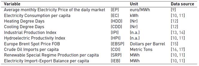
Herein after, information of the country in the data set is given through suffixes -P and -S, for Portugal and Spain, respectively.

3. Forecasting research methodology

Forecasting time horizons are not consensual in literature and vary in agreement with the primary objective of the analysis. Thresholds for electricity price forecasting may vary from a few minutes up to days ahead (short-term time horizons), from few days to few months ahead (medium-term time horizons) and months, quarter or even years (long-term time horizons), being the latest usually based on lead times measured in months. As previously introduced, the proposed analysis aims at forecasting electricity prices on a monthly basis ahead.

Numerous methods of forecasting electricity prices have been proposed over the last years. There are several modelling approaches, statistical models, multi-agent models, and computational intelligence techniques, which can be found in [³]. It is also noteworthy the growing use of hybrid models, combining those methodologies, as described in [¹⁸].

The forecast methodology in this work uses a statistical approach, which chiefly derived from classical load forecasting. Statistical methods forecast the current price by using a mathematical combination of the previous prices and/or previous or current values of the exogenous or independent variables. The main advantage of the price forecasting based on exogenous variables is that it allows system operators to interpret some physical characteristics in the electricity price formation. In this context, and despite a large number of alternatives, Multiple Linear Regression Model (MLRM) is still among the most popular forecasting approach and is the model adopted in the current analysis.

3.1 Multiple Linear Regression Model

The MLRM is a statistical model that assumes there is a linear relationship between the dependent or predictor variables, Y, and X independent variables, the latter being exogenous, explanatory, non-stochastic and observable variables, used to explain the variation of the variable Y. A model that comprises more than one independent variable is a multiple regression between a dependent variable and a set of n+1 independent variables assuming a linear form and stochastic because it includes an error term [¹⁹]. The Multiple Linear Regression Model is given by Equation (1), as follows:

where is the y-intercept, represents the parameters of the model, and is the error term.

A casual association is not assumed between dependent and independent variables. In this sense, the dependent variable, Y, depends on a set of n+1 known factors and an unknown factor, being an endogenous variable, explained, stochastic or random and observable.

Typically, the linear regression model uses the following assumptions [²⁰]:

• The regression mode is linear, as proposed in Equation (1);

• The regressors are assumed to be fixed or non-stochastic in the sense that their values are fixed in repeated sampling;

• Given the values of the independent variables, the expected value of the error term is zero;

• The variance of each error term, given the values of independent variables, is constant or homoscedastic;

• There is no correlation between two error terms, i.e., there is no autocorrelation;

• There are no perfect linear relationships among the dependent variables, i.e., there is no multicollinearity;

• The regression model is correctly specified.

Based on the assumptions mentioned above, the most popular method for parameters estimation, the Ordinary Least Squares (OLS), provides estimators which have several desirable statistical properties, such as [²¹]:

• The estimators are linear, which means that they are linear functions of the dependent variable, Y;

• The estimators are unbiased, which means that, in repeated applications of the method, on average, they are equal to their true values;

• The estimators are efficient, which means that they have minimum variance.

3.2 Measures of forecasting accuracy

The main purpose of the modelling and forecasting processes is to clearly discern the future values of the dependent variable, and the most important criterion of all is how accurately a model does this. The most familiar concept of forecasting accuracy is evaluated through the error magnitude accuracy, , which relates to the forecast error of a particular forecasting model, defined by Equation (2) [²²]:

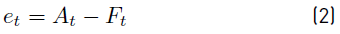
being the actual value and its forecast in the time period, t.

Although there are various measures of forecasting accuracy that can be used for forecast evaluation, in this work it is used the mean absolute percentage error (MAPE) expressed in generic percentage terms, computed by Equation (3) [²⁰]:

As stated previously in Section 3, electricity prices under analysis are based on a monthly temporal basis, for which data is significantly higher than zero. Under these circumstances, the MAPE measure performs satisfactorily on the forecasting accuracy evaluation.

4. Electricity price modelling and forecasting

4.1 Data sample and generic model

The modelling methodology adopted the historical data from January 2010 till December 2015, with a total of 72 observations. Data from 2016 year was used to validate the model, and data from 2017 and 2018 years were applied to produce the forecasts and to build the models, based on the previous validation from 2016 data, already working with 84 observations (January 2010 till December 2016).

The results were produced through GRETL statistical software (Gnu Regression, Econometrics and Time-series Library) for Windows.

The output model is no more than a representation of the relations between the variables at the same time set, according to Equation (1). Average monthly electricity price (EP) modelling and forecasting, for the Portuguese and Spanish markets, employs the econometric model given by Equation (4):

It should be noted that models for Portuguese and Spanish markets interrelate the electricity price with explanatory variables for each country.

4.2 Electricity prices modelling for Portugal

The results obtained for Portugal with the Multiple Linear Regression Model, estimated by the application of the Ordinary Least Squares Method for 2017 year are presented in Table 2.

Table 2 Performance measures of the estimated model for Portugal, 2017 year 

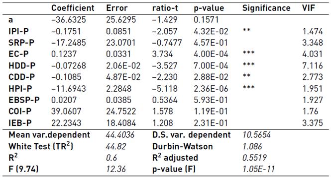
Notes: *, Significance of 10%; **, Significance of 5%; ***, Significance of 1%.

From the results obtained, the coefficient of determination is 0.6, which indicates that the independent variables explained about 60% of the variations that occurred in the electricity prices in Portugal. The adjusted coefficient of determination is 0.5519 which indicates that about 55% of the changes in electricity prices were explained by the variations in the independent variables. It is also possible to conclude:

• The autonomous component indicates that -36.6325 of the electricity prices for Portugal are not explained by independent variables. However, this variable does not reveal a statistically significant value;

• If the variables IPI-P, SRP-P, HDD-P, CDD-P, and HPI-P vary by one unit, the Electricity Price variable decreases. However, from those variables, only IPI-P, HDD-P, CDD-P and HPI-P reveal statistical significance;

• The variable electricity consumption per capita (EC-P) has a positive relation with the Electricity Price: if the first one varies one unit the later increases by approximately 0.1237 units. This variable is statistically significant, with a significance level of 1%;

• The variable COI-P has a positive relation with the Electricity Price: if the first one varies one unit, the Portuguese electricity price variable increases in 39.0607 units;

• From the analysis of the Electricity Import-Export Balance per capita (IEB-P), it has a direct relation with the Electricity Price, if the first one varies in one unit, the Portuguese electricity price variable increases in 22.2343 units;

• Regarding the F statistic (9.74), there is sufficient statistical evidence to verify that there are variables that assume values other than zero and, as previously mentioned, the variables included in the model explain satisfactorily the changes in Electricity Prices in Portugal;

• From the analysis of the violation of the basic hypotheses of the model, in terms of multicollinearity and based on the values of the Variance Inflation Factor (VIF), there is no violation of the basic hypothesis of multicollinearity, since the VIF values, for all variables, are lower than 10. It can be concluded that there is no dependence on explanatory variables;

• Regarding the residue analysis, normality was evaluated using the Kolmogorov-Smirnov test made through the statistic test 0.6701, with p-value=0.7351, which means that this model follows a normal distribution at a significance level of 1%, so this hypothesis is not violated. The mean is equal to μ= 5.0753E-15, i.e., approximately zero, from which the zero-mean hypothesis is also not violated E (μ)=0;

• For homoscedasticity, a constant variance of the error term was verified by the White test for heteroskedasticity and the test statistic TR ²= 45.6799 with test value ((54) > 45.6799) =0.7825. Because the test value is higher than 10%, it can be concluded that there is no violation of homoscedasticity, i.e., the variance is constant from observation for observation. There is no loss of the characteristics of OLS estimators, since they remain BLUE;

• The Durbin-Watson statistic=1.0863 lies in the zone of positive autocorrelation of the errors. Then, it can be concluded that there is an infringement of the independence of the error term and that this model suffers from autocorrelation of the errors. In order to correct the infraction hypothesis, the Cochrane-Orcutt test was applied. Accordingly, the following statistic was obtained: Durbin-Watson=2.0855, which is now in the zone of independence of the errors.

In order to be able to model and predict electricity prices for 2018 year, it was necessary to create a trend line from the price of electricity for Portugal and create 12 dummies (dm) or periodic auxiliary variables that represent each of the months of the year of 2018. These auxiliary variables were created as assistance to the model, due to the absence of data from the independent variables referring to the year 2018, from September 2018. In addition, to remove the trend component, a variable has been eliminated (for instance, dm2), and the least squares method was applied. The performance measures of the model are presented in Table 3.

Table 3 Performance measures of the model with periodic auxiliary variables for the Portuguese market, 2018 year 

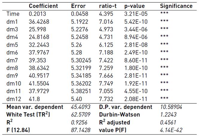
Notes: *, Significance of 10%; **, Significance of 5%; ***, Significance of 1%.

It is also necessary to verify that the obtained model for 2018 does not violate the infractions in order to be able to validate it. Based on the performance measures of the current model and regarding the violation of the model hypotheses, it can be concluded that:

• All auxiliary variables are statistically significant at a significance level of 1%;

• There is no violation of the basic hypothesis of multicollinearity, considering the low values of the Inflation Factor of the variance;

• Constant variance of the error term, by White test for heteroscedasticity, since the value of evidence is higher than 10%, there is no violation of homoscedasticity;

• The Durbin Watson statistic=1.2243 was found in the zone of positive autocorrelation of the errors, meaning that there is an infraction to the independence of the error term. To overcome the previously verified infraction, the Cochrane-Orcutt test was applied. Accordingly, the following statistic was obtained by Durbin-Watson=2.02538 which translates in independence of the errors.

4.3 Electricity prices modelling for Spain

Following the same methodology described in previous section, the model obtained for Spanish market, in 2017 year (presented in Table 4], presents a coefficient of determination of 0.5826 and indicates that the variables EC-S, HDD-S, CDD-S, HPI-S, IPI-S, EBSP-S, SRP-S, COI-S, IEB-S explain 58.3% changes of electricity prices in Spain during 2017 year. The adjusted coefficient of determination is 0.53, which indicates that about 53% of the changes in electricity prices in Spain are explained by the independent variables.

Table 4Performance measures of the estimated model for Spain, 2017 year 

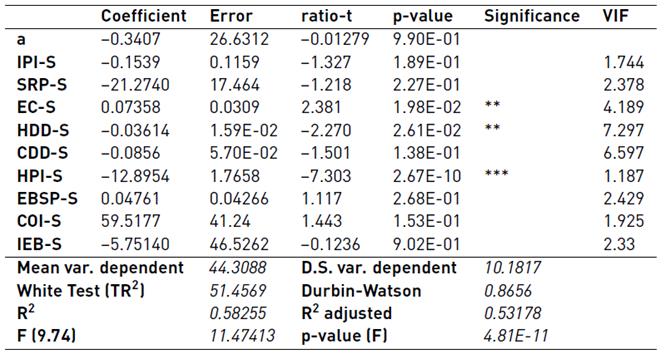
Note: *, Significance of 10%; **, Significance of 5%; ***, Significance of 1%.

Based on the results obtained and presented in the table above, it can be concluded that:

• The autonomous component shows that -0.3407 of electricity prices in the Spanish market are not explained by the independent variables. This variable is not a statistically significant variable;

• Variables IPI-S, SRP-S, HDD-S, CDD-S, HPI-S, and IEB-S have an inverse relationship with the Electricity Price. From those, only variables HDD-S and HPI-S are statistically significant;

• EC-S, EBPS-S, and COI-S have a positive relation with the Electricity Price but only the EC-S reveals to be statistically significant, at a significance level of 5%;

• Regarding F statistic F(9.74)=11.47413, with a test value lower than 1%, there is sufficient statistical evidence that there are variables that assume values different from zero and as previously mentioned, the variables included in the model explain in a satisfactory way the variations occurred in the electricity prices in Spain;

• The analysis of the infraction to the basic hypotheses of the model, considering the VIF, it is verified that there is no infringement of the basic hypothesis of multicollinearity (all variables present VIF lower than 10). There is no correlation between the explanatory variables;

• The test of normality of the residue performed through the statistic test 0.767096, with test value=0.68144, means that this model follows a normal distribution at a significance level of 1%, so this hypothesis not violated. The mean value is approximately zero, so the zero-mean hypothesis is also not violated E (μ) = 0;

• Constant variance of the error term, through the White test for heteroskedasticity and the test statistic, is higher than 10%, i.e., there is no violation of homoscedasticity.

Regarding the model and prediction of the electricity prices for the Spanish market, for 2018 year, following the same methodology stated in the previous section, the model performance measures are presented in Table 5.

Table 5 Performance measures of the model with periodic auxiliary variables for the Spanish market, 2018 year 

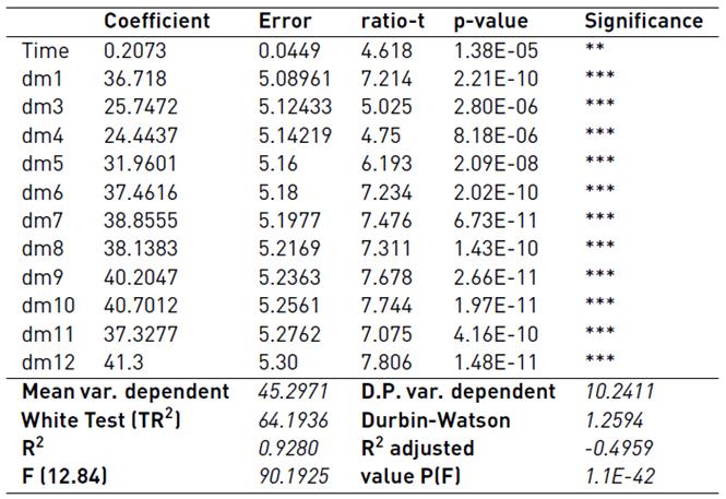
Note: *, Significance of 10%; **, Significance of 5%; ***, Significance of 1%.

From the statistical tables proposed by Durbin and Watson [²³], for 9 independent variables the lower bound (dL) is equal to 1.4173, upper bound (dU) equals 1.8876, 4-dU is equal to 2.1124 and finally 4-dL is equal to 2.5827. It was obtained the following Durbin-Watson statistic=0.865615, which lies in the zone of positive autocorrelation of the errors, meaning that there is an infringement of the independence of the term of error. Following the application of Cochrane-Orcutt test, a Durbin-Watson statistic=1.9481 is obtained, which satisfies the independence of the errors.

From the information presented in Table 5, the model for the Spanish market for 2018 year does not violate the infractions, validating it. All auxiliary variables are statistically significant with a significance level of 1%. Additionally,

• Regarding the analysis of multicollinearity, considering the VIF, it is verified that there is no violation of this hypothesis;

• White test has a test value higher than 10%, i.e., there is no violation of homoscedasticity;

• The Durbin-Watson statistic=1.2593 was obtained. This value is in the positive zone of autocorrelation of the errors, being necessary further analysis, using the test of Cochrane-Orcutt to verify if that the infraction can be solved. With the Cochrane-Orcutt test the following Durbin-Watson statistic=2.029 was obtained and, consequently, there is independence of the errors.

4.4 Forecasting results for Portugal and Spain

This section presents the forecasts for the Electricity Price, for each of the country’ markets under analysis, for 2017 and 2018 years, based on the models created and described in the previous sections.

To evaluate the accuracy of the prediction, it will be used the Absolute Percent Error (APE) and Mean Absolute Percent Error (MAPE). The assumed confidence interval to produce forecasts is 95%. The results obtained for the two models selected, with the previous described methodologies, and for the respective statistical measures/indicators are presented in Table 6 and Table 7, for Portugal and Spain, respectively.

Table 6 Electricity prices forecast for Portugal, 2017 and 2018 years 

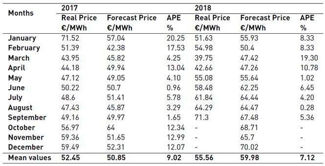
Regarding the Portuguese market [Table 6] and 2017 year, it can be observed that the difference between the actual and expected annual averages is € 1.6 and the MAPE is 9.02%. Forecasts for 2017 follow the behaviour of real historical prices. For 2018, and considering the known prices, that is, between January 2018 and September 2018, it is notorious that the forecast follows the same behaviour. The MAPE, evaluated for 9 months, equals 7.12%.

From the analysis of the data of average monthly electricity price for the Portuguese Market, considering the period of analysis from January 2017 to September 2018, it is verified that this indicates maximum values in the winter months, where variables such as EC-P and HDD-P are higher which may justify the increase in electricity prices. Extrapolating this analysis to the remaining periods, it is possible verify that the electricity prices register lower values for the summer months, where the EC-P is smaller. The minimum values of the electricity Prices are registered in March and April, for both years under analysis. This decrease in price is justified when the months have a very high HPI-P, from which higher-cost energy sources can be withdrawn from service, contributing to the decrease of the Electricity Price.

Table 7 Electricity prices forecast for Spain, 2017 and 2018 years 

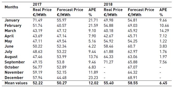
Regarding electricity prices for Spain [Table 7], it is observed that the forecast values for 2017 are higher, by € 1.95. The MAPE obtained for 2017 was 12.02%, higher than its counterpart from Portuguese market forecast and for the year 2018, about 6.45%. Analysing the year of 2017, it can be verified that the predictions follow the same behaviour of the original series, which allows trusting the model. With reference to the forecast of the average monthly electricity price for the Spanish market, maximum values are also found in winter months, where variables such as EC-S and HDD-S are higher. Similar to the results obtained for Portugal, it can be verified that the electricity prices register low values in summer months, when the EC-S is lower.

5. Conclusions

This paper presented a statistical model with explanatory variables for long-term electricity price forecasting in the Iberian electricity market. The establishment of such a reference model presents itself as an opportunity to interpret their components, intending to understand the complexity associated with price forecasting.

Regarding the Portuguese market, variables reflecting the production of goods (Industrial Production Index), ambient conditions (Heating and Cooling Degree Days), hydroelectric potential (Hydroelectric Productivity Index) and demand (Electricity Consumption per capita) are statistically significant. As far as the Spanish market is concerned, only the variables Hydroelectric Productivity Index, Heating Degree Days and Electricity Consumption per capita, are statistically significant. Therefore, it is possible to state that the electricity price in the Iberian electricity market is mainly interrelated with the inputs demand, ambient weather conditions and generation capacity.

From the analysis of the performance of the developed models, the model for the Portuguese electricity market for the year 2017, presents better results than the model applied for the Spanish electricity market. Regarding the forecast models for the year 2018, the model developed for Spain gives the best performance and the lowest MAPE.

The developed modelling suggests that factors with higher impact in the Portuguese electricity market may not be the same factors which influence the neighbouring Spanish market, even though they share to the same energy market.

The quality of the estimated models validates the use of statistical or causal methods, such as the Multiple Linear Regression Model, as a plausible strategy to obtain causal forecasts of electric energy prices in medium and long-term electricity price forecasting.

Future work will explore other approaches beside regression models to compare forecasting performances, strengths and weaknesses of different statistical techniques. A comparison with autoregressive-type time series models, relating the electricity price to its own past, and also a hybrid approach, adding the effect of the most notable exogenous variables should also be performed.