English (pdf)
 Article in xml format
 Article references
 Send this article by e-mail
 Cited by SciELO
  Cited by Google
  Similars in
SciELO
Similars in
SciELO  Similars in Google
 Permalink
1. Introduction
The World’s population is moving from rural to urban areas and it is expected that this trend will continue. The number of inhabitants in cities will be about 75% of the World’s population by 2050 [1].
The fast demographic growth, together with the concentration of the population in cities and the increasing amount of daily waste are factors that push to the limit the ability of waste assimilation by Nature. This fact has forced the authorities to examine the cost-effectiveness and environmental impact of our economic system.
The linear structure of our economy has reached its limits and the natural resources of our planet are drained. Thus, a more sustainable model of economy is needed. For example, the circular economy [2, 3], which consists in the transformation of our waste into raw materials, proposing a new paradigm for a more sustainable future.
The unsustainable development of countries has created a problem due to the unstoppable waste generation. In addition, there are hardly any technological means to make an optimal management of the waste collection process. Nowadays, the solid waste collection is carried out without a previous analysis of the demand, i.e. following a manually defined route. This approach has severe limitations, one of the most important is the variability in the amount of waste that needs to be picked up. This is especially critic in the case of selective collection (plastic, paper, glass,...), where the waste volume is smaller than in the organic case. Thus, when dealing with recyclable waste, the planning of the optimal collection routes is even more influential.
An alternative to tackle the planning of the collection routes is to determine which containers should be collected. Note that the recyclable waste collection process represents 70% of the operational cost in waste treatment [4]. Thus a reduction in the number of unnecessary visits to semi-empty containers will save money! We aim to provide an alternative to predict if a container should be collected or not. Particularly, we propose to predict the filling level of the waste containers (all the containers involved in the operation at once) using a Recurrent Neural Network (RNN).
RNNs are top-notch at predicting time series, however as all Deep Learning (DL) techniques the selection of an appropriate network design is a tough task [5]. The use of automatic intelligent tools seems a mandatory requirement when addressing the design of RNNs, since the vast possible RNN architectures that can be generated defines a huge search space. In this sense, metaheuristics [6] emerged as efficient stochastic techniques able to address hard-to-solve optimization problems. Indeed, these algorithms are currently employed in a multitude of real world problems, e.g., in the domain of Smart City [7-13], showing a successful performance. Nevertheless, the use of such a methodology in the domain of DL is still limited [14].
On the other hand, real-world problems present many challenges, from technological issues to political restrictions. In our particular problem, there is an interesting problem that arises when dealing with the prediction of the filling level: uncertainty. Following previous works [15], we distinguish two types of uncertainty, reliability against noise and robustness. The latter measures uncertainty caused by imprecision of the decision variables of the solution, which is not relevant for our problem because solutions can always be implemented precisely. The former measures uncertainty which may come from many different sources such as sensory/human measurement errors as it is the case of the historical data of filling level of the waste containers. Therefore, in this study, we propose to study whether RNN could provide reliable solutions when provided with noisy/faulty data.
In this article, we extend the ideas presented by [16]. Particularly, using a hyper-parameter technique based on evolutionary computation, we design and train an RNN that predicts the filling level of the containers of a whole city. Then, we study the behavior of this approach when faced with prediction under uncertainty. To validate our proposal, we analyze a real-world case consisting of more than two hundred waste containers located in a city in Spain, and we compare our results against the ones presented by [17].
As a summary, in this study:
We define a deep neuroevolutionary technique to automatically design an efficient RNN.
We use our proposal to design and train an RNN that predicts the filling level of the waste containers of a real city and benchmark our results against the state-of-the-art.
We study the RNN approach for predicting under uncertainty.
Therefore, the main contribution of this work in contrast to the previous work [16] is the analysis of the behavior of deep neuroevolution and RNN when faced with uncertain data.
The remainder of this paper is organized as follows. The next section briefly reviews the state-of-the-art of smart waste management. Section 3 discusses about the use of DL to predict the waste generation rate. Section 4 presents a deep neuroevolutionary approach to design an artificial neural network-based predictor of the filling level of the waste containers. Section 5 presents the experiments carried out, results, benchmark, and analyses. Finally, Section 6 outlines our conclusions and proposes the future work.
2. Smart waste management
The waste collection is a process with uncountable variants and constraints which have led to a multitude of studies in recent years due to its importance. The works in the literature could be classified, among other ways, according to the waste type that is treated: residential waste commonly known as garbage [10, 18], industrial waste where customers are more dispersed and the amount of waste is higher [19], recyclable waste [20] increasingly important for our society, where the collection frequency is lower than organic waste and hazardous waste where the probability of damage is minimized [21].
In the municipal solid waste collection [22], the authorities need global studies to quantify the waste generated in a period of time to be able to manage them. Particularly, the waste generation forecasting for Xiamen city (China) inhabitants was studied by [23]. The main difference with our approach is the granularity of the object under study. They predict the amount of waste produced by the whole city, in contrast, we predict every single container in a city (i.e. a disaggregated prediction of the whole city). This supposes a considerable increase of the complexity of the problem that is solved, because it is necessary to consider multiple aspects such as the location, the customs of the citizens, the population density of the area, etc. In the same research line, the impact of the intervention of local authorities on waste collection has also been studied [24], being this relevant in the medium-long term.
Regarding the location where the collection takes place, there exist multiple variants of the problem. There are communal collections where the local authority identifies a place shared by the community [11, 25], in most cases a local waste facility for recycling. In the other side we found the kerbside collection [26] where the household waste is collected from individual small containers located near each house. The intermediate case studied here is the analysis of containers that give service to several streets and blocks of flats [27].
In previous works [17, 28] the authors used machine learning techniques to predict the filling level of a container. Particularly, the authors used Linear Regression, Gaussian Processes and Support Vector Machines for regression to predict each container individually. In this work, we present a unique RNN able to generate predictions for the whole set of containers instead of creating and training individual predictors for each container.
3. Deep learning for waste generation prediction
In this study, we focus on waste generation prediction by applying DL based on specific type of artificial neural networks (ANN), RNN. As other ANNs, this type of networks are composed of multiple hidden layers between input and output layers. RNNs incorporate feedforward and feedback connections between layers to capture long-term dependency in an input. Thus, RNNs have successfully applied to address learning applications which involve sequential modeling and prediction as natural language, image, and speech recognition and modeling [29]. In turn, they have been applied in Smart Cities problems that require time dependent prediction [14].
We apply supervised learning, which consists in an iterative process that requires a training data set (N input-output pairs). As this study deals with the prediction of the filling levels, the inputs are the current filling level each container and the outputs are the next (future) filling levels. Thus, for each input, the ANN produces an output (i.e., a tentative future filling rate) which is compared to the expected output by using an error (cost or distance) function. Then, a procedure is applied to reduce this error by updating the network until a given stop criteria is reached [30].
Minimizing such learning error is a tough task. Backpropagation [31] (BP), a first-order gradient descent algorithm, is the most widely used method to address such issue. In order to apply BP on RNN, the network has to be unfold [32], i.e., the network is copied and connected in series a finite number of times (known as look back) to build an unrolled version of the RNN.
Large ANNs (as unfolded RNNs) suffer from overfitting to the training data set, i.e., the error on the training set is driven to a very small value, but when unseen new data is presented to the network the error dramatically increases [33]. In order to address this issue, a technique called dropout, which consists in including a stochastic procedure to the training process, is applied [34].
The accuracy and the generalization capability of the RNN prediction depends on a set of configuration hyper-parameters: number of layers, number of hidden units per layer, activation function, kernel size of a layer, etc. Thus, a promising research line in DL proposes to find specific hyper-parameters configurations for an ANN to improve its numerical accuracy [35, 36]. The results demonstrated that selecting the most suitable hyper-parameters for a given dataset provides more competitive results than using generalized networks.
Since training an RNN is costly (in terms of computational resources) and the number of RNN architectures is infinite (or extremely large if we impose restrictions to the number of hidden layers or neurons), we are enforced to define a smart search strategy to find an optimal RNN.
Among the many potential optimization techniques to find efficient ANN hyper-parameterization, a few authors have already applied metaheuristics [37, 38]. However, these solutions cannot be directly applied to deep neural networks (DNN), i.e. ANNs with one or more hidden layer, due to the high computational complexity of DNNs. Recently, new solutions specifically defined to address hyper-parameter optimization of DNNs by using metaheurisitcs are emerging: the deep neuroevolutionary approaches [5, 14, 39-41], showing competitive results in finding parameters that improve the accuracy and minimize the generalization error.
In this study, we focus on applying a deep neuroevolution approach to address the generation of container filling predictions. Our optimization method deals with the next main RNN parameters: the look back (i.e., how many times the net is unfold during the training), the number of hidden layers, and the number of neurons for each hidden layer.
4. Deep neuroevolutionary architecture optimization
In this section, we present the details of our proposal. First, we formally state the architecture optimization problem, and then we outline our deep neuroevolutionary approach to solve the problem.
4.1 Architecture optimization
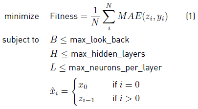
Optimizing an ANN consists in finding an appropriate network structure (architecture) and a set of weights to solve a given problem [30]. Particularly, we can analyze the suitability of an ANN by measuring its generalization capability, i.e. the ability to predict/classify new (unseen) data.
In our case, we are interested in optimizing the architecture of an RNN. Therefore, we decided to train an RNN using BP (i.e. we are finding an appropriate set of weights given a network structure) and measure the mean absolute error (MAE) of the predicted values against the observed ones.
Equation (1) states the problem of finding an optimal architecture as a minimization problem, where N corresponds to the number of samples in the testing data set (X,Y), zi stands for the predicted value of the i-th sample, and yi corresponds to the ground truth of the i-th sample. Note that the RNN is fed with already predicted data x, and that the architecture is constraint by B, H, and L.
4.2 Deep neuroevolution
To solve the problem stated in Equation (1) we designed a deep neuroevolutionary algorithm based on the (1 + 1) Evolutionary Strategy (ES) [6] and on the Adam weights optimizer [42]. Our proposal is presented in Algorithm 1.
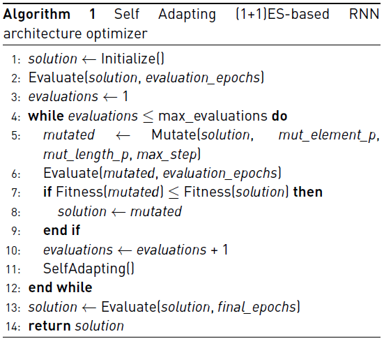
A solution represents an RNN architecture and it is encoded as an integer vector of variable length, solution=< s 0, s 1, …, s H >. The first element, s 0 ϵ [1; max_look_back], corresponds to the look back, while the following elements (s j , j ϵ [1;H]), correspond to the number of Long Short-Term Memory (LSTM) cells of the j-th hidden layer, subject to s j ϵ [1; max_neurons_per_layer] and H ϵ [1; max_hidden_layers]. Note that the number of hidden layers is defined by the length of the vector. The number of neurons of the output layer is defined accordingly to the inputed time series, i.e. we add a dense layer (fully connected) with a number of neurons equal to the number of dimensions of the output.
First, the Initialize function creates a new random solution. Then, the Evaluate function computes the Fitness of the solution. Specifically, the solution is decoded (into an RNN), then the net is trained using the Adam optimizer [42] for evaluation_epochs epochs using the training data set and finally the fitness value is computed using the testing data set.
Then, while the number of evaluations is less or equal than max_evaluations, the evolutionary process takes place. Starting from a solution, the Mutate function generates a new mutated solution, which is later evaluated. The Mutate function consists in a two step process applied to the inputed solution. In the first step, with a probability equal to mut_element_p the j-th element of the solution is perturbed by adding a uniformly drawn value in the range [-max_step,max_step]. In the second step, with a probability equal to mut_length_p the length of the solution is modified by copying or removing (with equal probability) an element of the solution. Before returning the new solution, a validation process is performed to assure that the mutated solution is valid (i.e. its values complies with the restrictions).
Next, the fitness of the original solution and the mutated one are compared. If the fitness of the mutated is less or equal than the original solution, the mutated replaces the original solution.
As the last part of the evolutionary process, a SelfAdapting step is performed to improve the performance of the evolutionary process [43]. Particularly, if the fitness of the mutated solution improves the original one, then the mut_element_p and mut_length_p values are multiplied by 1.5, in other case these probabilities are divided by 4 [43]. In other words, if we are not improving, we narrow the local search space. On the contrary, while the solutions are improving (in terms of the fitness), we widen the local search space.
Finally, the evolved solution is evaluated (using final_epochs to feed the number of epochs of the training process) and returned.
5. Experimental study
We implemented our proposal in Python 3, using the DL optimization library dlopt [44], and the DL frameworks keras [45] and tensorflow [46]. Then, we (i) selected a data set to test our proposal, (ii) optimized an RNN to tackle the referred problem, (iii) compared our predictions against the state-of-the-art of urban waste containers filling level prediction, and (iv) studied the suitability of the solutions found to predict under uncertainty.
5.1 Data set: filling level of containers
The data set analyzed in this article is the one used in [17, 28], a real case study of an Andalusian city (Spain), where we highlight the benefits of our approach, being effective and realistic at the same time. Our case study considers 217 paper containers from the metropolitan area of a city. The choice of an instance of recycling waste (paper) is more attractive than a organic waste collection to show the quality of our approach because most paper containers do not need to be collected everyday like the organic waste, so they have a high variability in collection frequency.
In order to study the reliability of our approach under uncertainty we propose a synthetic benchmark of instances derived from the original data set. We selected a percentage p of random days where the filling data of all containers have errors, which may come from a) sensors errors or b) the loss of the data. From these two source of errors, we generate two types of instances. To represent the former source of errors (a) we generate random values between 0 and 100 to fix errors in data, we call it random. For the latter one (b) we use zeros to represent the loss of data, so we call it zeros. Combining the percentage of days with errors (p = 5; 10; 20) and the type of errors (zeros or random) we generate 6 synthetic instances.
5.2 RNN optimization
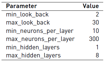
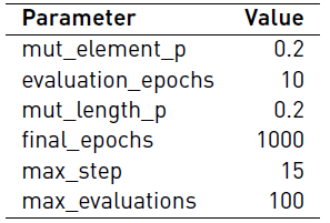
We executed 30 independent times our deep neuroevolutionary algorithm considering the combinatorial search space defined in Table 1, using the data set described above, the parameters defined in Table 2, and a fixed dropout equal to 0.5. We use an 80% of the data to train the networks and the remainder data to test their performance (i.e., computing the fitness).
The initial setup of the algorithm is taken from the related literature [14]. Considering that our proposal performs a self-adapting step, we did not perform a tuning of the parameters of the algorithm.
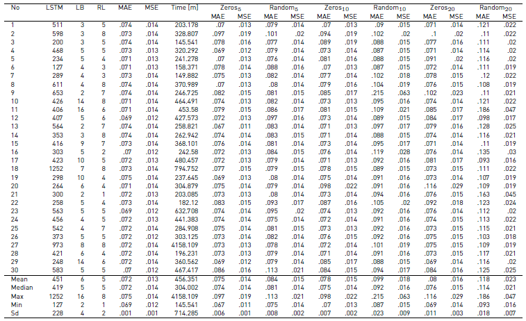
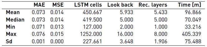
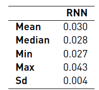
Table 3 summarizes the results obtained. The MAE, the mean squared error (MSE), the total number of LSTM cells, the look back, and the number of recurrent layers correspond to the statistics computed over the final solutions (30 RNN trained). We will refer to the solution returned by the algorithm as solution. The time corresponds to the statistics computed over the total time, i.e. the sum of the computation time of all the architectures evaluated, including the solution. The time is presented in minutes.
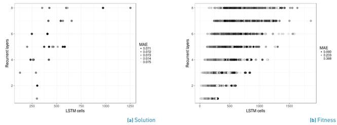
The results show that the algorithm is robust in regard to the MAE (and the MSE), however there is a noticeable variation in the architectures and in the time needed to compute a solution. We analyze the solutions and all the architectures evaluated during the optimization to get insights into the relation between the architecture and the error. Figure 1a presents the architectures (number of LSTM cells and layers) of the solutions along with their respective MAE and Figure 1b shows the same for all architectures evaluated. A small MAE (a darker dot) is desirable. It is important to remark that the MAE presented in both figures is not comparable, because in both cases the number of training epochs is different, therefore the results are expected to differ (at least in their magnitude).
It is quite interesting that the solutions are very diverse (see Figure 1a), and that most of them use less than 500 LSTM cells. This is more interesting if we consider that the maximum allowed number of LSTM cells given the problem restrictions (see Table 1] is equal to 2400 and that many architectures evaluated have more than 500 LSMT cells (see Figure 1b).
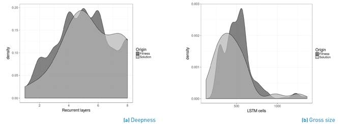
To continue with our analysis, we ranked all the architectures evaluated (excluding the solutions) into deciles and selected the top one (i.e. the best architectures evaluated). Then we plot the density distribution of the number of recurrent layers (see Figure 2a) and of the total number of LSTM cells (see Figure 2b). We also plot the density distribution of the solutions in both figures. The results show that both densities are relatively similar, therefore we intuit that there is an archetype that better suits to the problem. However, further analysis is required to validate this intuition.
5.3 Prediction benchmark
In order to continue with the evaluation of our proposal, we benchmark the predictions made by the RNN against the results published in [17, 28]. In order to compare the approaches we compute the “mean absolute error in the filling predictions of the next month” (MM) using the solutions given by our algorithm, i.e. we predict a whole month using an RNN and summed up the predictions per container, then we compute the mean absolute difference between the predicted values and the ground truth. Table 4 summarizes the results of the MM computed using the solutions. Note that the MM results are better than the MAE (see Table 3].
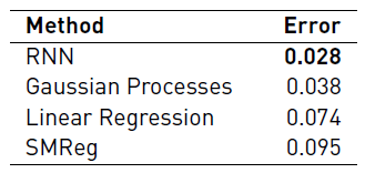
We selected the median solution (in regard to the MM) and compared the results against the ones presented in [17, 28]. Table 5 presents the benchmark in terms of the prediction error. In that previous work, the authors proposed three time series algorithms used for forecasting the fill level for all containers. Particularly, they used techniques based on Linear Regression (LR), Gaussian Processes (GP), and Support Vector Machines for Regression called SMReg.
The results indicate that our proposal exceeds its competitors. Moreover, we performed a non-parametric Friedman’s Two-Way Analysis of Variance Ranks Test that revealed RNN as the best algorithm, followed by the algorithm based on GP, the LR, and the SMReg as last algorithm in the comparison. Regarding the statistical significant differences, the values have been adjusted by the Bonferroni correction for multiple comparisons. There are significant differences between each pair of algorithms except for the particular comparison between LR and SMReg. Thus, the RNN is significantly the most competitive method according to the MM.
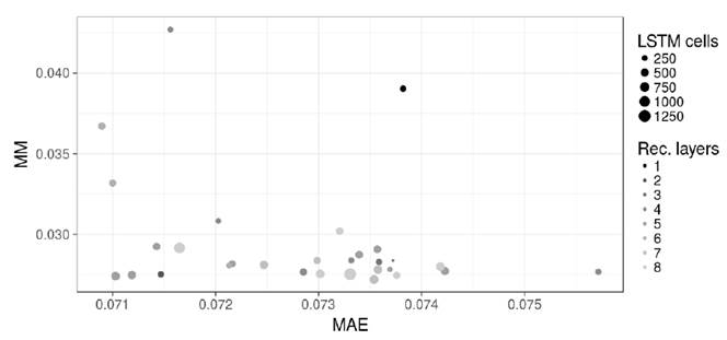
Finally, to relate the results presented in this subsection (see Table 4] to the ones presented in the previous subsection (see Table 3] we plotted the relation between the MAE and the MM (please refer to Figure 3]. The figure also includes the architecture of the solutions (number of LSTM cells and number of recurrent layers). Something that caught our attention is that there is not an apparent linear relation between both metrics presented in the plot, however the summarized results presented for both metrics (see Tables 3 and 4] are robust in regard to the referred error measurement.
5.4 Prediction under uncertainty
Following up with our experimentation, we studied the reliability of the solutions found. Particularly, we re-trained (Section 5.2) the solutions found (30 RNNs) using the synthetic dataset described previously.
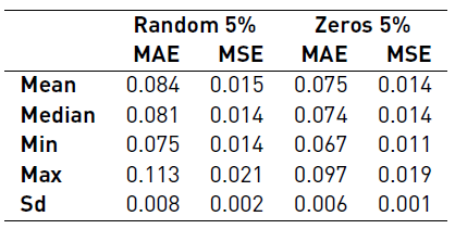
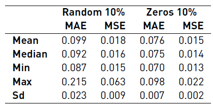
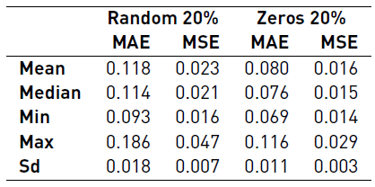
Tables 6, 7 and 8 summarize the results of the reliability benchmark. At a glance, we notice that the overall results worsen as the uncertainty increases, as it is expected. Basically, the quality of the data has a direct impact in the accuracy of the predictions.
We also observed that losing data (i.e. replacing measurements with a zero) is not as important as having random errors. In other words, it is preferable to have a missing data (non-functioning sensor) than having an imprecise measurement (or faulty sensor). This particular insight presents a new challenge (or problem) to real waste management companies, because it is clear that a non-functioning sensor is easy to found, however a faulty one might be hard to detect.
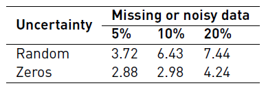
In order to compare the predictions under uncertainty against the predictions made by our competitors [Table 5], we selected a solution per combination (random/zeros and percentage) whose MAE is equal to the median and we computed the MM. Table 9 presents the described results. As expected, the results show that adding uncertainty to the data has a negative impact on the MM. Moreover, a missing datum (zeros) has less impact than a random noisy datum. On the other hand, if the uncertain data represent less than the 5%, the RNN still beats all its competitors [Table 5]. Note that the results shown in Table 5 do not consider uncertain data.
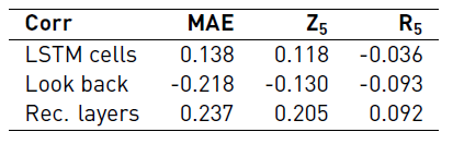
In order to gain insights into the relation between the performance and the architecture, specially in regard to the variation of the uncertainty, we computed the Pearson correlation between the MAE and the architecture definition of each solution. Particularly, we computed the correlation between the total number of LSTM cells, the look back, and the number of recurrent layers, and the MAE, MAE with a 5% missing (zeros) or faulty data (random). Table 10 presents the correlations computed. The results show that there is a small correlation between the variables. Therefore, further analysis is needed to conclude that there is a relation between the performance and the architecture in this case (adding uncertainty to the dataset). Please refer to Table 11 in Appendix for a detailed version of the results.
6. Conclusions and future work
Deep neuroevolution has emerged as a promising field of study and is growing rapidly. Particularly, the use of Evolutionary Algorithms to tackle the hyper-parametrization optimization problem is showing unprecedented results, not only in terms of the performance of the designed networks, but also in terms of the reduction of the computational resources needed (e.g., the configurations are evaluated using a heuristic, therefore not all configurations are actually trained [47, 48]).
In this study, we present a deep neuroevolutionary algorithm to optimize the architecture of an RNN (given a problem). We test our proposal using the filling level of 217 waste containers located in Andalusia, Spain, recorded over a whole year and benchmark our results against the state-of-the-art of filling level prediction. Our experimental results show that an “appropriate” selection of the architecture improves the performance (in terms of the error) of an RNN and that our prediction results exceeds all its competitors.
In regards to the quality of the predictions under uncertainty, the result show that the quality gets worse as the percentage of missing or faulty data increases. Nevertheless, the median RNN (not the best) is able to outperform all its competitors (using correct data) even when the RNN uses an instance which has 10% of missing data. In addition, by analyzing in detail the RNN results’ under uncertainty, we conclude that it is preferable to have missing data than imprecise data coming from a faulty sensor. This fact should be considered when we receive an outlier from a sensor.
As future work, we propose to explore train-free approaches for evaluating a network configuration. Specifically, we propose to study the use of the MAE random sampling [47, 48] to compare RNN architectures, aiming to reduce the computational power and the time needed to find an appropriate architecture.