


 English (pdf)
 Article in xml format
 Article references
 Send this article by e-mail
 Cited by SciELO
  Cited by Google
  Similars in
SciELO
Similars in
SciELO  Similars in Google
 Permalink
1. Introduction
Smart City (SC) has emerged to solve the problems of population growth and urbanization [1]. However, this new concept of city must experiment changes to enable this evolution. The reality indicates that cities are evolving, for example in [2], 15 UK cities are analyzed, and the results are that carbon dioxide emissions do not grow/decrease linearly.
SC must adapt its existing infrastructures. These new SC need to solve existing problems in transport, energy, energy efficiency, integration of renewables, mobility, citizenship, etc. A critical infrastructure is the electricity grid, as shown in [3]. In addition, as shown [4], the rapid increase in population and population flows require a complete modernization of existing infrastructures (electricity, water, gas, etc.).
Energy efficiency is key and fundamental in the SC, and buildings are one of the most important infrastructures in the city. These buildings, like the city, must evolve, and they must integrate renewable sources and improve their energy efficiency [5]. This new building concept, called Smart Building (SB), will be responsible for increasing the efficiency and sustainability of the SC, since it will integrate renewable sources and other good practices [6-8].
As already mentioned, SC aims to improve efficiency at all levels. This increase in efficiency may affect the advanced programming of SB behavior [9]. Energy efficiency also refers to the sending of information through the SC [10-11]. Another important aspect of energy efficiency has to do with the reduction of peak demand and energy savings, as presented [12] through its new algorithm.
As exposed in [13], the integration of large-scale renewable sources in cities is a reality. But this integration must be done in an efficient way, as mentioned in [14], and this efficient way refers to the way to install and improve the production of energy. Integration can be understood in a massive but small-scale way, as presented by the authors in [15], where small-scale integration is with photovoltaic (PV) and solar. PV numbers during the last years show an undeniable landmark in renewable energies.
The world added more capacity from solar PV than from any other type of power generating technology.
In this sense, the increase in efficiency in renewable systems is critical, as they reflect in [16, 17]. Therefore, this work is focused on demonstrating the increase of efficiency in the PV systems integrated in SC, since these renewable plants will be subject to numerous shadows (solids, obstacles, etc.). The use of optimizers at the PV module level will increase the efficiency of the overall system. The present paper is an extension of the research displayed in the Iberoamerican Congress of Smart Cities (ICSC-CITIES 2018) [18]. The authors have developed several shadow scenarios, increasing the tests performed from six to eight, which have been validated with simulations and within a real environment. Electrical structure of the module simulated in LTSpice and electric connection of optimizers has been introduced. Additionally, the increment in production for each scenario has been analyzed and an economic study of the installation of DC optimizers considering three different electricity price scenarios has been carried out. In this way, the system performance has been tested when shadows affect cells on different circuits and in different percentages. The paper is divided as follows: section 2 presents a theoretical review, section 3 explains the methodology used, section ?? shows the results, section ?? discusses the results and section ?? presents the conclusions of the work.
2. Theoretical review
The performance of PV modules is inevitably decreased due to the different working conditions of each of the panels. The PV system output power will be reduced as a consequence of mismatch effects and environmental factors caused by partial shading, soiling, dirtiness, mismatch between PV cells generated during their manufacture or ageing mismatching, differences in the orientations and inclinations of solar surfaces, differences in temperature or irradiance in the modules. A lot of the available energy would be wasted since the shaded PV cells would be acting as passive charges and they would limit the output current of the unshaded ones [19]. These effects lead to the weakest PV cells determining the output power of the whole string of modules. Therefore, additional potential benefits of distributed power electronics include increased design flexibility by allowing mismatched or longer strings of PV panels, improved monitoring, and increased system availability [20].
In order to avoid this, DC-DC converters on PV module level can be added. These devices, commonly known as power optimizers, are mounted in each single module and minimize the impact that the different factors have on the performance of PV systems. Additionally, it allows testing the behavior of each module by means of communications included into the electronic device, facilitating the operation and maintenance of PV arrays [21]. This is really beneficial in the cases of big PV plants, in which there are a large number of PV modules connected, because they help to identify whether a PV module is working well. In case of absence of optimizers, it would be possible to identify the array in which the failure is located, but it would be more difficult to detect the single module or modules which fail. A quick detection of failures would avoid energy losses due to faults on the PV system.
Another appropriate application for this technology is the case of Building Integrated Photovoltaic (BIPV) systems, in which the environmental factors can be very significant in contrast with open-space plants. While a large PV plant is designed with the single aim of optimizing energy production, the goal of a BIPV system is not only electricity generation but also the achievement of aesthetical and functional objectives from an architectonic point of view [19]. The optimal orientation and inclination of BIPV systems are practically impossible, as well as avoiding partial shadows. Furthermore, having all the modules tested in BIPV systems is an enormous advantage, because in this case, the access to PV panels can be very complex and it will incur heavy maintenance costs.
As a result of shadows or other failures, the P-V curve shows two Maximum Power Points Tracking (MPPT) values, one global and one local [21]. MPPT controllers find and maintain operation at the MPP using an MPPT algorithm. The modular converters incorporate this function. The literature proposed many of these algorithms. For instance, some MPPT methods such as fractional open circuit voltage and fractional short circuit current are simple to implement with moderate level of accuracy. The commonly used perturb & observe (P&O) technique produces oscillation around the maximum power point with a possibility of failure under partial shading condition. Other appliances employ PV power forecasting models to compute the reference value of the maximum PV power to be tracked by a direct power control scheme which of composed of a SEPIC converter [22].
The investigations through this topic started at the end of the 20th century [23]. First of all, in 1992, it was studied the incorporation of DC-AC converters in each module. In this way, each module will have a small inverter and the grid connection of the PV modules will be carried out directly in AC current, so the mismatch and environmental factors will not affect from one module to the rest of them. Some authors affirm that the peak efficiency of the system is 89% and that they have a lifetime of approximately ten years [24]. Nonetheless, it has some important disadvantages which inspire the study of alternative solutions. Firstly, it is quite difficult to reach efficiently and reliably the grid voltage from the output power of a module. Moreover, the use of several micro-inverters implies the duplication of protections and AC filters to offer the same quality and safety than a central inverter, which leads to a more expensive solution. Different micro-inverters efficiencies are analyzed in [25], in which a test circuit that can be used as efficiency measure to analyze and compare different features of micro inverters is designed.
The necessity of micro AC inverters to boost the DC voltage and invert it leads to a lower efficiency and higher cost than DC-DC converters. Therefore, the implementation of DC-DC converters has been the main alternative studied during the last decade. During the first years of the 21th century, the first application of this concept was proposed. In 2004, a cascaded DC-DC converter connection of PV modules was proposed [26]. It offers the advantages of modular converters approach without the cost or efficiency drawbacks of individual DC-AC grid connected inverters. Later experimental results show an efficiency of approximately 95% [27]. Nevertheless, the performance of converters depends on the operating conditions of the PV system along with the performance characteristics of the converter [20]. There are many different topologies which vary according to the complexity of circuits, stress on used components and quality of input and output power. Generally, a single-inductor, single-switch boost converter topology and its variations exhibit a satisfactory performance in the majority of applications where the output voltage is greater than the input voltage. The performance of the boost converter can be improved by implementing a boost converter with multiple switches and/or multiple boost inductors. The two inductor boost converter exhibits benefit in high power applications high input current is split between two inductors, thus reducing power loss in both copper windings and primary switches. Furthermore, by applying an interleaving control strategy, the input current ripple can be reduced [28]. More recent developments carried out point to newer DC-DC technologies with low cost and high reliability. In the delta-conversion concept [29], the converters are only active when differences between substring and module output powers occur. This reduces the operation time and thereby increases the reliability.
3. Methodology
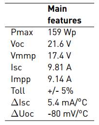
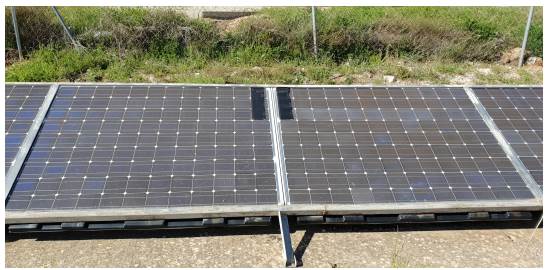
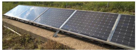
Experiments have been performed in the PV field of the Campus Duques de Soria, University of Valladolid. Two strings of eight Isofoton I-159 modules, with the same mechanical configuration and orientation, compose this PV field. The main characteristics of the modules used in the tests are shown in Table 1.
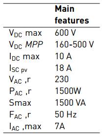
The first string is directly connected to a string inverter, SB 1.5-1VL40, which the main characteristics are shown in Table 2.
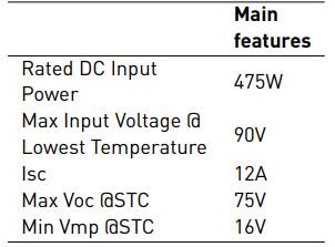
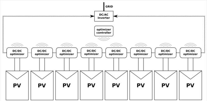
On the other hand, the second string has optimizers TIGO TS4-O installed in each module, which characteristics are reviewed in Table 3. The eight optimizers are connected in series to a second inverter identical to the first-string inverter [Table 2], as showed in Figure 1.
Eight different tests have been studied to determine the influence of DC-DC optimizers in the production in case of shading. Different diagrams of the six shadings configurations are further analyzed in the results section. Then, the scenarios are indicated:
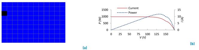
Test 1:one module affected, the shaded part will be 80% of three cells of the same circuit, leaving the rest of the module in standard conditions.
Test 2: one module shaded in each string, affecting 50% of the surface of nine cells.
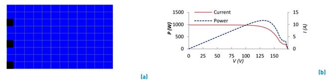
Test 3: one module shaded in each string with 100% of the surface of thirty-six cells belonging to the same circuit.
Test 4: four modules of the string affected. In each module a line of 12 cells, belonging the same circuit, is shaded at 50% of its surface.
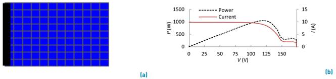
Test 5: whole string shaded in the same percentage as test 4, 12 cells in each module shaded at 50% of its surface.
Test 6: one module affected, covering 80% of nine cells in the same column, affecting all three circuits.
Test 7: one module affected, covering 80% of three cells in different circuits.
Test 8: one module shaded, covering 100% of one single cell.
As an example, Figure 2 shows the shading configuration in test number 1 and Figure 3 the shading configuration in test number 4. As an example, Figure 2 shows the shading configuration in test number 1 and Figure 3 the shading configuration in test number 4.
All shading configurations have been simulated in LTSpice using the methodology proposed in reference [21], in order to obtain the theoretical IV curves to make possible the evaluation. Additionally, the real IV curves of the strings for each shading configuration have been experimentally obtained using the HT SOLAR IV-400 TRACER. The dimensions of the module used are presented in Figure 4a and the electrical structure of the module simulated in LTSpice in Figure 4b.
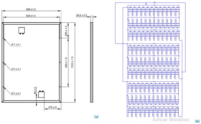
Figure 4 Isofoton I-159 modules dimensions (a) and electrical structure of the module simulated in LTSpice (b)
Finally, all the results downloaded from the string inverters and the optimizers have been analyzed and compared considering the resultant theoretical and experimental IV curves of each shading configuration and the analysis is presented in the results and discussion section.
4. Results and discussion
In this section, we explain the two types of experiments that have been carried out. Firstly, computer simulations with LT Spice software and secondly field simulations in the PV field of the Campus Duques de Soria (University of Valladolid) are displayed. Additionally, the results of the IV curve experimental tests in the field are shown and compared with LTSpice simulations.
4.1 LTSpice experiments
LTSpice is a SPICE simulation freeware for analog circuits endowed with schematic capture and a wave form viewer. This software has been used to simulate the IV curves for each shading test proposed, which are presented in this section.
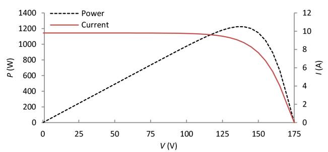
Benchmark
In benchmark simulation there is no shaded cells in order to see clearly the ideal graphics of both power and current, as showed in Figure 5. Power curve has a maximum point at 1223.8W
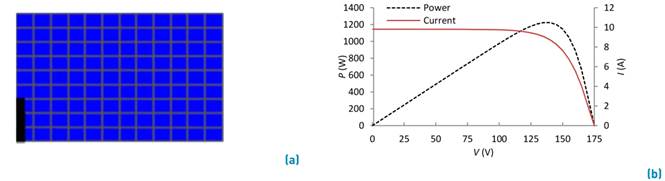
Test 1
With only one module affected, the shaded part will be 80% of three cells of the same circuit, leaving the rest of the module in standard conditions [Figure 6a). In this simulation, two MPP appear clearly [Figure 6b) with similar values of 1048.5 W and 1049.2 W.
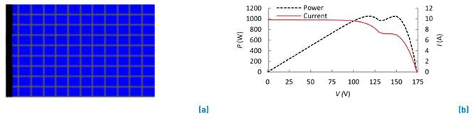
Test 2
It continues having only one module shaded in each string, affecting 50% of the surface of nine cells [Figure 7a) belonging to three different circuits. Figure 7b shows how the power curve is affected by this new type of shadow, resulting in two MPP with values of 1048.5 W and 784.9 W.
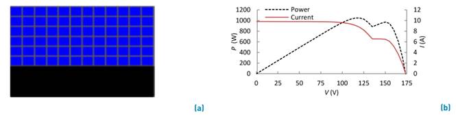
Test 3
Only one module shaded, one circuit 100% affected (36 cells belonging to same circuit, Figure 8a). In Figure 8b first MPP in 1048.9 W remains equal as test 2 but the second MPP rises up to 972 W.
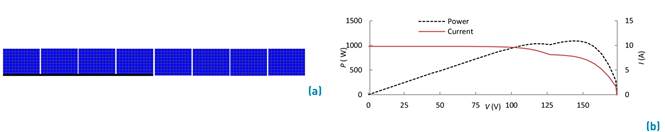
Test 4
First one affecting 4 modules. In each module a line of 12 cells, belonging the same circuit, is shaded at 50% of its surface [Figure 9a). In Figure 9b, power graph exhibits two MPP at 1035.8 W and 1092 W.
Test 5
Continuing with the shadows of test 4, test 5 has the whole string shaded in the same way as the previous test, 12 cells in each module shaded at 50% [Figure 10a). This power curve graph lowers the first MPP to 838.5 W but maintains the maximum in 1033.1 W [Figure 10b).
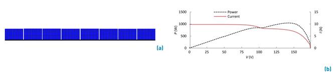
Test 6
This test concerns only to one module covering 80% of nine cells, affecting all three circuits [Figure 11a). Although tests 2 and 6 are similar, the shading difference of 30% causes the lowest MPP to fall to 306.5 W, with the high remaining at 1048W [Figure 11b).
First test affecting non-consecutive cells in one module, with an 80% of its surface shaded. [Figure 12a). First MPP has a value of 1060 W and second one lowers its value to 325 W [Figure 12b).
4.2 Field experimentations
Tests were developed from May to June, with duration of one week for each, the shadow position was changed every Monday. The day in which the shadows are changed is not considered in the tests, so there are six full days for each one.
Atypical weather (strong storms, cloudy and windy days) in certain days of tests 3, 4 and 6 generated graphics full of maximums and minimums instead of the standard production graph. Production data is monitored by each inverter, one mark every 5 minutes.
In order to simplify nomenclature, strings are numbered “String 1” and “String 2”. String 1 worked with optimizers and String 2 worked without them.
There are natural shadows affecting both Strings in late afternoon and first evening hours. Figures along this section present the power in each time of the day, in contrast to the previous section in which simulated IV curves were showed. This is because field experiments presented in this section are performed with the objective of calculating the difference of production using optimizers, in a specific period of time, and thus it is dependent on the external conditions during that timeframe. On the other hand, IV curves in the previous section were presented to show how the different defined shadow configurations affect the production. However, two experimental IV curves have been included at the end of the section, which are compared with the simulated ones.
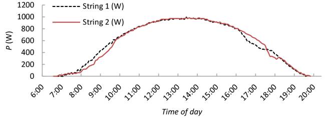
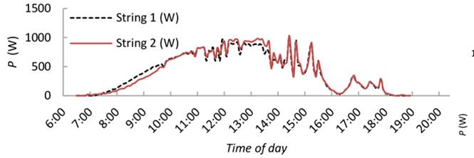
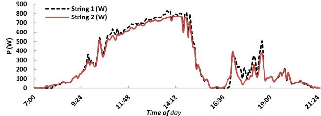
Benchmark
Five days of benchmark data with similar production graphics in sunny days [Figure 14] and disparate production charts on cloudy days [Figure 15], left two recognizable patterns common to all days: string 2 starts sooner than string 1 and string 1 produces more than string 2 in the first hours of the morning. In cloudy days, string 1 has more difficulty reaching some of the production peaks after the cloud leaves [Figure 15].
Test 1
Same shadow pattern as simulations with LTSpice, one module shaded with 80% of three cells of the same circuit, leaving the rest of the string in standard conditions [Figure 6a).
One cloudy and windy week collecting data show results like Figure 16, full of maximums and minimums. Still there is the same pattern: String 1 starts later but rises first in early hours of the day.
Test 2
One module shaded in each string, affecting 50% of the surface of nine cells as showed in Figure 7a. This week string 1 had strange graphs that we attribute to some technical error or a bad configuration of the inverter [Figure 17].
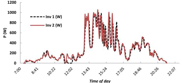
Test 3
One module shaded in each string with 100% of the surface of thirty-six cells belonging to the same circuit. This was another atypical stormy week with late afternoon heavy rain periods. Figure 18 displays String 2 higher production on cloudy periods before the storm.
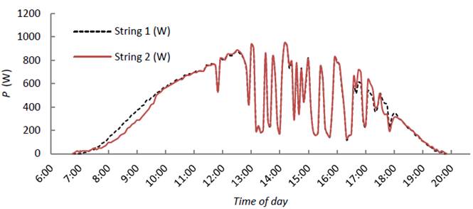
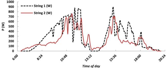
Test 4
This week only 4 of 8 modules were affected with one line of 12 cells belonging to the same circuit, shaded at 50% of its surface [Figure 19]. Another stormy week full of moments of sun left production peaks and long intervals below 400 W, as seen on Figure 19.
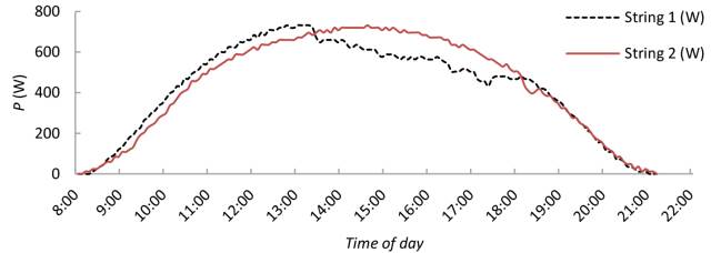
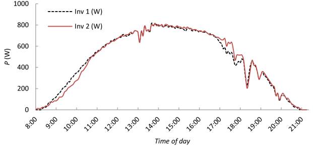
Test 5
This test has the whole string affected, 12 cells in each module shaded at 50% [Figure 10a). Graphs are very similar from string 1 to string 2 with only one common pattern: string 2 starts first but string 1 produces more in the first hours of the day [Figure 20].
Test 6
With a similar pattern of test 2, test 6 has strong differences between the production of the two Strings which increases its value considering that it was a rainy week. Figure 21 shows a typical rainy day on Test 6 week.
Test 7
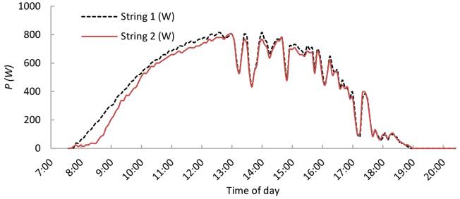
During all the days in which the test 7 was carried out, it is verified that string 1 has better production than String 2. The weeks of test had cloudy days and others partially sunny, Figure 22 shows a partially sunny day.
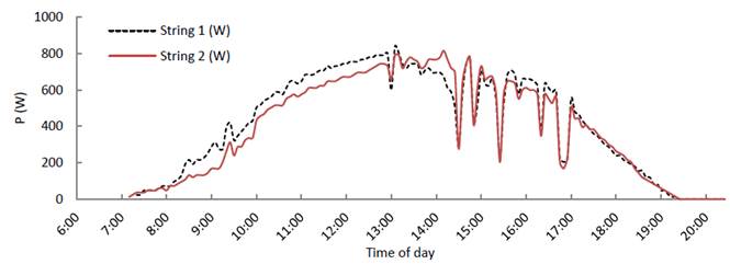
Test 8
All test 8 week had partially sunny days and, like other tests, String 1 has better production than String 2 in every single day. Figure 23 displays an example of a sunny day with some intermittent clouds.
To obtain more conclusive results, it is necessary to have more data, therefore, be able to carry out tests for a longer time; but tests with longer measurement time implies controlling the climatic conditions (having little variation), and this is not possible. For this reason, the tests carried out have been limited in time. However, the comparison of the data has been made between the two strings of each test separately and although the meteorological conditions were not the most suitable, available data of the two strings of each test can be compared without any issue, as they have been taken in equal conditions.
On almost every test day, the graphs showed that the power delivered by String 1 is greater than the supply by String 2, even though some tests were carried out with adverse weather, stormy and rainy weeks, etc.
In the first few minutes of the day, the String 2 starts its production before but then the optimizers generate an acceleration to the power delivered by the String 1 in the early hours of the day when the sun is still far from its zenith leaving a positive count clearly in favor of optimized String.
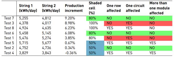
Table 4 shows the daily production averages of each test with the percentage of shade and common characteristics are added.
After these groupings, it is shown that the relationship between the increase in production and the rest of the characteristics is centered on the percentage of the shaded cell. The increase in production decreases with the decrease in shade.
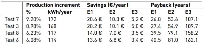
It has been performed an economic analysis for the fourth test with the highest production increment, test 7 (9.20%), test 3 (8.98%), test 8 (6.23%) and test 6 (6.08%), with the objective of obtaining the payback of the optimizers installation. The yearly electricity production of the installation of eight modules (1.27 kW) of the University has been obtained using the PV calculator of the Joint Research Centre [30], resulting in 1,870 kWh/year. Three different electricity price scenarios have been considered; the approximate current price of 0.06 €/kWh (E2), double price (E1=0.12 €/kWh) that has been a common price recently (from 2010 to 2015) and half price (E3=0.03 €/kWh), which could be a realistic scenario in the near future, considering actual tendency of electricity price decrement. Finally, the price of the installation of the eight optimizers and the central receptor has been 552.8 €. Results obtained are showed in Table 5. As it can be seen, results show that the payback varies from 26.8 years for test 7 configuration and scenario 1 to 162.1 years for test 6 configuration and scenario 3. As it can be seen, actual tendency of photovoltaic technology price decrement leaves no room for optimizers installation at their current price, but they could be a feasible option if their price decreases, if the electricity price increases or in case of having a different configuration of shadows responsible of a higher production increment using DC optimizers.
Table 5 Economic analysis of the installation of DC optimizers in three different electricity price scenarios (E1= 0.12 €/kWh, E2= 0.06 €/kWh and E3= 0.03 €/kWh)
Additionally, to the analysis of the production introduced, it has been performed the real IV curves of the strings for each shading configuration using the HT SOLAR IV-400 TRACER. Some of these results are presented in this section. Figure 24 shows the IV curve of Test 4 configuration which is really similar to Figure 6b: Both have one lower MPP (at low voltage and high current value) and then one higher MPP (at high voltage and low current value). The big difference between them relies on the first MPP, as simulation points it at 1035.8 W but the real measure sets it at 700W. This is mainly caused by the degradation of the module, which has been exposed during several years as detailed in the methodology.
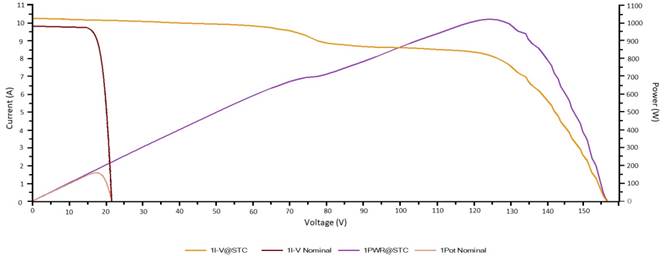
Figure 24 Test 4 shadow configuration IV and PV Curve. Orange-purple curve presents the IV-PV curve of the string of eight modules applying shadow of test 4. Brown-pink curve presents the IV-PV curve of one module applying shadow of test 4
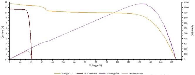
Another example of the panel degradation can be seen in the Figure 25. Corresponding to Test 5, can be contrasted with Figure 10b. First MPP on simulation was at 838.5 W but due to material degradation the PV curve, first MPP in real conditions is at just 350 W.
5. Conclusions
Energy efficiency is key in the SC, in which integration of renewable sources is a reality. Specifically, PV technology is the most promising of all, since its integration in buildings and public spaces is simple. In this sense, the increase in efficiency of the deployed technology is fundamental. In case of PV, the presence of shadows can cause the performance drop of energy delivery. Intelligent devices such as those presented in this work (DC-DC optimizer) can make PV technology better in production.
This research shows how the String of PV modules equipped with DC-DC optimizers delivers a higher power in seven out of the eight tests carried out, despite the absence of optimal weather conditions, noting that the greater percentage of the cell is shaded, the more work optimizers will do. The results must be taken into account in those locations where there are shadows, which may affect the PV modules. This paper includes an economic study of the installation of DC optimizers considering three different electricity price scenarios, resulting in a minimum payback of 26.8 years. Finally, it is proposed as an interesting future work performing a comparison of the efficiency with a string of modules equipped with micro inverters. Future work could extend actual research using other DC converters manufacturers, to study their influence in production.

