


 Inglês (pdf)
 Artigo em XML
 Referências do artigo
 Enviar este artigo por email
 Citado por SciELO
  Citado por Google
  Similares em
SciELO
Similares em
SciELO  Similares em Google
 Permalink
1. Introduction
According to the Mining and Energy Planning Unit of Colombia (UPME) [1], 52% of Colombian territory is not connected to the local grid and the energy demand is going to duplicate in the next 40 years. Furthermore, 75% of the energy is supplied by hydroelectric power that could have a negative impact on the environment [1]. Nowadays, there is only one wind farm that produces 19.5 MW in the country [1], but the wind direction changes constantly due to Colombian topography. So, there is a need of developing wind power solutions capable of using this fluctuating resource in order to diversify the energy portfolio. This research is the first one in analyzing the wind power density at the Chicamocha’s canyon, the second largest canyon worldwide, which needs to improve its surroundings infrastructure to promote tourism [2]. The electrical grid at the canyon is not stable due to its topography, and local community need a sustainable source of energy that does not impact the environment, and ensures an economic growth in the tourism industry. Therefore, one of the main purposes of this research is to determine the feasibility for installing Vertical Axis Wind Turbines (VAWT) there.
The performance of a VAWT relies principally on its airfoil, which generates lift and drag forces that take advantage of the wind kinetic energy to produce torque at the shaft of the turbine. Airfoil design and selection is an important task that depends on three main topics: wind flow conditions, airfoil shape, and modeling. Currently, Darrieus VAWT blades design are based on lift aerodynamic force and uses the commercial NACA0018 airfoil. A previous research [3] developed a new airfoil for these turbines: the DU06W200 airfoil, which overcomes the aerodynamic performance of the NACA0018. In that work, experiments and modeling of the airfoil based on Blade Element Momentum (BEM) theory are proposed. Nevertheless, the Reynolds numbers analyzed are higher than those observed in the Chicamocha’s Canyon. Furthermore, the drag coefficient calculated through their developed software, RFOIL, overestimates the experimental values. Then [4] compared the airfoils DU06W200 and NACA0021 in terms of energy performance and aerodynamic forces. The analysis is done with the commercial Computational Fluid Dynamics (CFD) software “Fluent 6.3.26” for a Re = 5:3 × 10⁴ applying the “k-" Realizable” [5] turbulence model. However, a validation of the turbulence model is not presented, the pressure coefficient distribution is not conclusive and nor lift or drag values are presented. The NACA0018 airfoil has been studied previously too for wind turbines, e.g. [6] analyzed that airfoil performance for horizontal wind turbines at the wind speed of 32 [m/s], but the application differs from the one this research is looking. Also experimental tests were conducted such as [7] focused on transition over the NACA0018 airfoil at a Reynolds number of 1 × 10⁵ and analyzed the shear layer distribution. Other CFD simulations of the NACA0018 airfoil are available such as [8-10], however the Reynolds numbers analyzed are not in the range of Chicamocha’s canyon needs. The [11] research meet the requirements of the current research but only one angle of attack is analyzed. Therefore, this research complements the previous studies by increasing the range of Reynolds numbers analyzed for the DU06W200 airfoil, providing further information about the aerodynamic global coefficients and analyzing the performance of both airfoils under different attack angles.
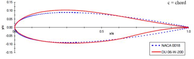
This work has a double purpose. First, determining the feasibility installation of VAWT at Chicamocha’s canyon. Second, selecting the airfoil for the wind turbine blade that presents highestaerodynamic efficiency under the wind flow conditions found at Chicamocha’s canyon. The present study applies a CFD numerical approach by means of the free software “OpenFOAM”. Turbulence is solved by the one equation RANS model developed by Spalart-Allmaras [12]. The geometry of the airfoils studied, i.e. DU06W200 and NACA0018, can be seen in Figure 1.
2. Methodology
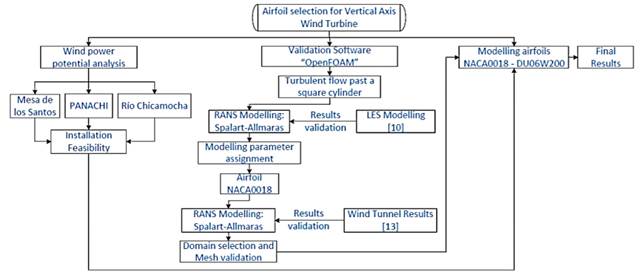
Figure 2 shows the research scheme applied in this study. The work is composed by two components: firstly, a wind density potential study of Chicamocha’s canyon, and secondly, a CFD modeling aimed to compare the airfoil’s performance under realistic conditions to suggest one for the wind turbine blades.
2.1 Installation feasibility of VAWT´s at Chicamocha’s canyon
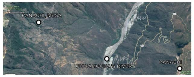
The Chicamocha’s canyon national park, known as “PANACHI”, monitor constantly the wind velocity at the canyon to control the cableway safety installed at the location. The administration of the park provided to this research the historical of the data from the year 2009 up to 2012. It possesses the wind velocity magnitude at the places known as “Mesa de los Santos”, “Chicamocha’s River” and “PANACHI” [Figure 3]. The historical includes daily information at three schedules: 8:00 am, 12:00 pm and 5:00 pm.
By using the collected data, the feasibility of installing a VAWT is analyzed. The mentioned wind turbines are suggested for the location since the blades do not need to be pointed towards the wind direction to be effective. Moreover, its structural and aesthetic principles have improved power generation in turbulent flows [4, 14].
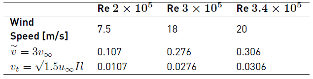
The wind energy potential of the canyon is analyzed by using the mass conservation principle (Equation (1)]:
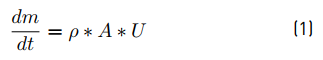
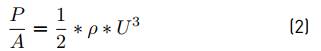
Where ρ is the air density, U the velocity and A is the swept area. Then, the wind energy potential, P, can be expressed as kinetic energy per time unit as (Equation (2)]:
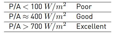
In this research the criterion presented in [14] is taken into account to establish how significant the wind energy potential is at a selected location [Table 1].
2.2 Aerodynamic study
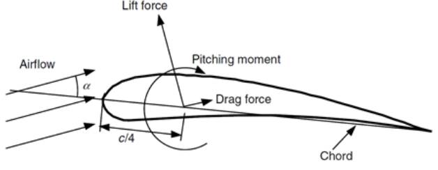
The wind flow incidence over the airfoil generates a force distribution along its surface, which can be decomposed into lift and drag force [Figure 4].
These parameters are defined through their dimensionless coefficients: Lift coefficient, c l , and drag coefficient, c d, defined in Equation (3) and (4) respectively.
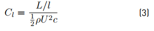
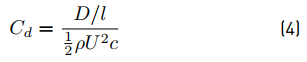
Where L/l and D/l indicate the lift and drag force per unit span of the wing respectively, and c the airfoil’s chord. By using the Dynamic Similitude concept [14] the airfoil’s performance depends on the attack angle, the Mach and the Reynolds numbers.
2.3 CFD airfoil studies
Different researchers have improved airfoil’s performance for wind turbines by means of wind tunnel tests and theoretical studies [1, 11]. Nevertheless, these efforts are time-consuming and need high technology laboratories [14]. Therefore, the use of simulation tools has become crucial to develop a wide range of aerodynamic technologies. For fluids, the CFD use has increased in the past decades since the modeling of the flow allows the analysis of microscopic scales that cannot be easily captured in experimental tests.
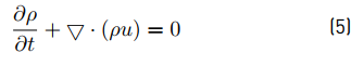
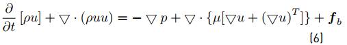
The incompressible fluid flows are governed by the Navier Stokes equations of mass conservation (Equation (5)] and momentum (Equation (6)].
These equations are nonlinear and can be handled by adopting an iterative approach. Nevertheless, there is none explicit equation for computing the pressure field that appears in the momentum equation. Moreover, solving general fluid flows requires an algorithm that can deal with the pressure-velocity gradient coupling.
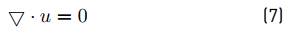
In the present research the flow is assumed to be steady, turbulent and incompressible, therefore the continuity and momentum equations (written in conservative form) are expressed in Equations (7) and (8).

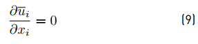
The turbulence regime can be solved either Direct Numerical Simulation (DNS) or Indirect Numerical Simulation (INS). The DNS solves each temporal and spatial fluctuation scale of the vortex energy cascade, but the computational cost is large enough to make it unfeasible for solving industrial applications due to the high-density meshing and short temporal steps needed [15]. On the other hand, an INS applies either a temporal averaging (RANS) or a spatial average fluctuation, to model the vortex generation and uses a turbulence model to close the system of equations. That make INS feasible for industrial applications as the current research requirements. A RANS filtering is applied to the governing equations of the flow leading to Equations (9) and (10).
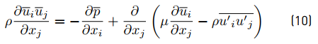
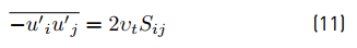
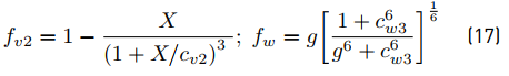
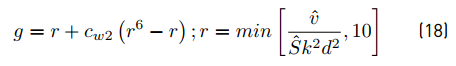
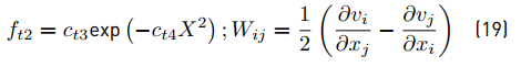
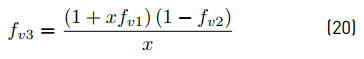
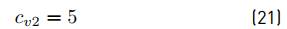
The term  is the Reynolds stress tensor and represents correlations between fluctuating velocities. In order to model it, the Spalart Allmaras-fv3 (S-A fv3) turbulence model is selected due to literature recommendations [16] and a turbulence model validation described in section 3 . The model is described as follows (Equation (11) - (21)]:
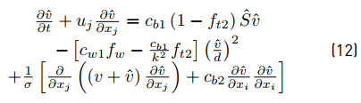

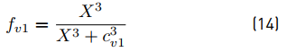
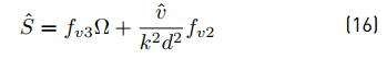
Where Ω = √2W ij W ij is the vorticity magnitude and d the distance to the nearest wall. Finally, is given:
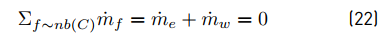
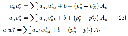
By using the Finite Volume Method (FVM), the partial differential equations representing conservation laws (Equations (9) and (10)] are transformed into discrete algebraic equations. The FVM is a conservative method as the flux entering into a given volume is identical to the outflow of the adjacent volume. In addition, it can be formulated at unstructured polygonal meshes as the unknown variables are evaluated at the centroids of the volumes and not at their faces. The method starts with the discretization of the geometric domain, i.e. divide the domain into non-overlapping finite volumes. Then, the partial differential equations are discretized into algebraic equations by its integration over each discrete volume. Finally, the system of algebraic equations is solved to compute the dependent variable at each of the control volumes. By using this FVM method, some terms in the conservation equation are turned into fluxes evaluated at the faces of the finite volumes. The discretized form of the momentum and mass conservation equations can be seen at Equations (22) and (23).
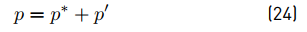
Equation (23) can be solved only when the pressure field is given or estimated. Unless the correct pressure field is employed, the resulting velocity field will not satisfy the relation. Therefore, an initial velocity field (u*, v*, w*) is calculated based on a guessed pressure distribution (p*) to start the iterations. Then, a new value of pressure (p) is updated from Equation (24).
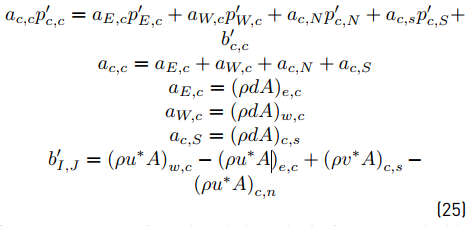
Where p’ is described at Equation (25).
Once the pressure is updated, the velocity is corrected with Equations (26)-(28).

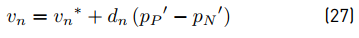

The described process corresponds to the Semi-Implicit Method for Pressure-Linked (SIMPLE) algorithm, which can be summarized as [16]:
Guess the pressure field p*.
Solve equation 23 to obtain u*, v*, w*.
Solve the p’ using equation 25.
Calculate p by adding p’ to p*.
Calculate u, v, w from their started values using equations 26-28.
Solve the discretization equation for other ϕ’s (such as temperature, concentration, and turbulent quantities) if they influence the flow field through fluid properties, source terms, etc.
Treat the corrected pressure p as a new guessed pressure p*, return to step b) and repeat the whole pressure until convergence is reached.
2.4 OpenFOAM modeling description
Different tests are made and compared with the literature to verify the mathematical models used. The type of boundaries established can be seen at Table 2.

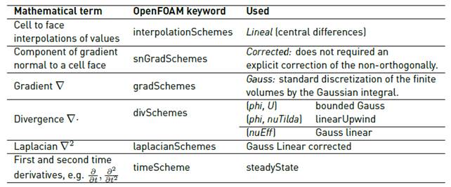
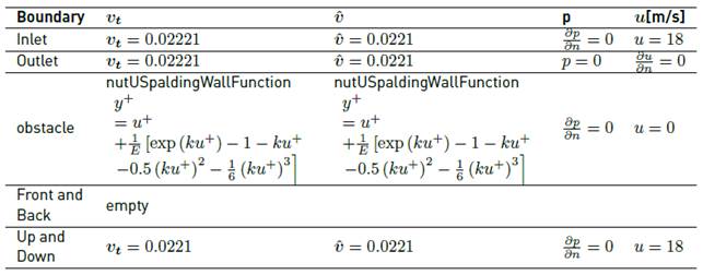
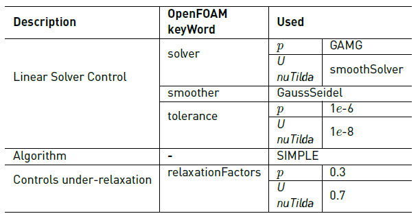
The numerical schemes are shown in Table 3. The boundary conditions and initial values of the variables are described in Table 4. Finally, the equations solvers, tolerances, and algorithms are shown in Table 5.
3. Discussion and analysis of results
3.1 “Mesa de los Santos” wind speed measuring
The annual average wind speed range from 5 up to 7 [m/s], giving a maximum wind power density of 450 [W/m 2 ]on February and a minimum of 180 [W/m 2 ] on July [Figure 5].

3.2 Chicamocha’s river wind speed measuring
At this location, wind flow accelerates due to mountains that surround the river, which acts as a nozzle directing the wind to a smaller section [Figure 6].

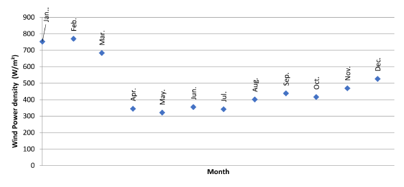
This effect is confirmed by the wind speed measured at the location, with peak value of 8.8 [m/s] and peak wind power density of 770 [W/m 2 ] as Figure 7 shows.
3.3 National park of Chicamocha (PANACHI) measurement
The maximum wind speed value is found in January with a value of 5.7 [m/s] and wind power density of 180 [W/m 2 ].Figure 8 shows the results.
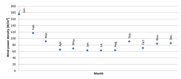
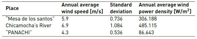
Table 6 summarizes the annual average wind speed and wind power density of the three locations. In brief, the feasible place for VAWT locations is at Chicamocha’s river due to its high average wind speed, 6.9 [m/s].
3.4 Validation and verification
Comparison between RANS and LES of turbulent flow past a square cylinder confined in a Channel
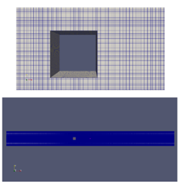
A square cylinder confined in a channel is simulated using different turbulence models to select the one that most approaches to literature results [17]. The influence of the mathematical simplifications and the SIMPLE algorithm is also analyzed. The domain used is shown in Figure 9.

The fluid properties are incompressible flow, Re: 3 x 10³, steady state, 2D and blockage ratio of 20%. A uniform velocity profile with a thin boundary layer thickness of 6% of channel height is necessary to replicate the case [17]. The boundary conditions used are the same as Table 4, modifying the initial values of the variables according to the fluid properties mentioned.
A Cartesian orthogonal mesh is used and refined at the boundaries of the obstacle, i.e. cube, as Figure 10 shows. Velocity components and turbulent fluctuations are averaged in time and in the cross-stream direction.
At Figure 11, the mean streamwise velocity along the centerline is shown for different simulations varying the mesh density. The results are compared with the literature [17] (black line). This comparison is performed to find the mesh independence, which is at 5 x 10⁵ cells, giving an average difference around 12% and standard deviation of 0,283. Therefore, the “simpleFoam” algorithm is validated for the Spalart-Allmaras fv3 turbulence model.
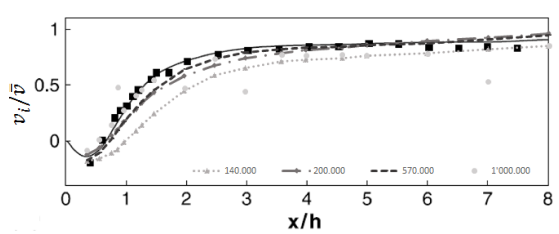
Figure 11 Mesh independence: Mean streamwise velocity profile along the centerline (■ and black line - literature [17]
By using the same modeling conditions and a mesh distribution of 5 x 10⁵ volumes, different turbulence models were analyzed: k-W SST, k-E Launder-Sharma and Spalart-Allmaras fv3. The results shown at Figure 12, concludes that Spalart-Allmaras fv3 model keeps the most accurate distribution in comparison with literature.
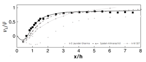
Figure 12 Turbulence models comparison: Mean streamwise velocity profile along the centerline (black line: literature [17])
DU06W200 modeling comparison between simpleFOAM and RFOIL software
The RFOIL software used in [3] based on BEM theory is compared with the current CFD results for Re = 5 x 10⁵, α = 0°, c = 0.25 [m] and free transition. To ensure a develop flow that reaches the airfoil, a channel length of 36c upwind, 44c downwind and a blockage ratio of 20% is designed [Figure 13].

A Cartesian orthogonal mesh is used and refined at the boundaries of the airfoil [Figure 14]. In addition, different meshes densities are analyzed for the Spalart-Allmaras fv3 turbulence model [Figure 15].
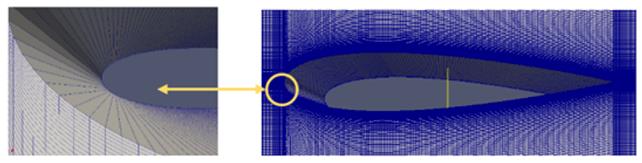
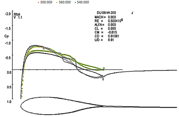
Figure 15 DU06W200 RFOIL and CFD data for Re = 5 x 10⁵, α = 0° (black line: literature [3], color lines: present)
The Figure 15 shows no significant variation after the mesh density of 3.6 x 10⁵ volumes. The CFD results follow the pressure distribution showed by the RFOIL software with an average difference of 15%. At high Reynolds numbers, RFOIL has problems to predict airfoil characteristics, e.g. it overestimates the maximum lift coefficient [3]. Such variation might be presented due to the lack of accuracy found at the trailing edge of the airfoil, where the turbulence model is sensible to vortex variations. Therefore, the CFD simulations will be used as the reference model.
NACA0018 validation with experimental tests
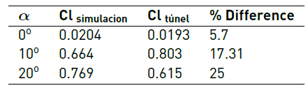
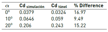
The numerical results are validated by comparing the lift and drag coefficients from the literature [7]. The airfoil is simulated under three different angles of attack: 0°, 10°, and 20°. The chord length (c) of the airfoil is 0.25 [m] and a Reynolds number of 3 x 10⁵ Results are shown in Table 6, Table 7 and Table 8. The boundary conditions are the same mentioned at Table 3. The ‘nutUSpaldingWallFunction” provides a turbulent kinematic viscosity condition when using wall functions for rough walls, based on velocity, using Spalding's law to give a continuous nut profile to the wall (y+ = 0).
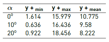
Wind flow behavior of the airfoil NACA0018 is shown in Figure 16.
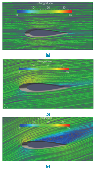
Figure 16 Wind velocity vectors over the airfoil at different angles of attack: (a) 0°, (b) 10° and (c) 20° [Author]
The implemented turbulence model accuracy is acceptable, presenting a maximum variation of 17% in comparison to the wind tunnel tests [7].The higher performance of the airfoil is found at the attack angle of 10°, where the lift and drag coefficients ratio has the greatest value: 10.3 approximately. Figure 17 shows a greater acceleration of the flow produced around the airfoil for an angle of attack of 0°, but as the angle of attack increases, the flow separation moves towards to the leading edge at the upper surface. It produces large vortex perceivable at the angle of attack of 20° at the trailing edge, which results in higher drag.
3.5 Results
Airfoils NACA0018 and DU06W200: performance analysis for Reynolds numbers between 2 x 10 5 and 3.4 x 10 5
This part analyzes the Reynolds number influence on the global aerodynamic parameters of each airfoil by using the FVM under the Spalart-Allmaras fv3 turbulence model. Similar grid size is adapted to each airfoil for this study. The modeling conditions are α = 10°, c = 0.25[m] and the fluid properties mentioned in Table 10.
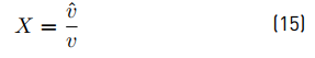
Where ῦ is the modified turbulent viscosity and v is the turbulent viscosity. The drag and lift coefficients are used in order to analyze the performance of the airfoils. The values can be seen at Table 11.
Table 11 Lift and drag coefficients from the airfoils NACA0018 and DU06W200 under different Reynolds numbers [Author]
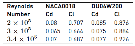
It can be concluded under the same Reynolds number, the lift coefficient of the DU06W200 airfoil overcomes in 23.3% the one from the NACA0018. As the Reynolds number increases, the lift coefficient increases too and the performance of the DU06W200 corresponds to the expectations of [3] design.
3.6 Airfoils modeling under Chicamocha’s canyon wind speed
The wind speed is the highest found at the analyzed locations, i.e. Chicamocha’s river (u = 6.93 [m/s]). The chord length of the airfoil, Reynolds number and angle of attack are defined at following: c=0.25[m], Re = 1.19 x 10⁵ steady-state regime and α =10°.

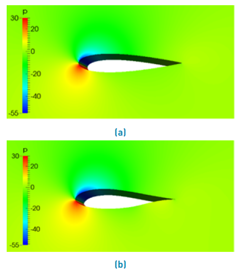
Figure 17 shows that wind speed at the leading edge of the airfoil DU06W200 is greater than NACA0018, confirming the airfoil optimization developed by [3]. Therefore, the cambered airfoil DU06W200 generates a high-pressure peak followed by a sharp fall of its values, as Figure 18 shows. This phenomenon produces turbulent flow quickly since the boundary layer cannot follow the pressure increase [3].
A consequence of the mentioned effects is quantified at the lift and drag coefficients presented in Table 12.
Table 12 Lift and drag coefficients of the airfoils NACA0018 and DU06W200 under Chicamocha’s canyon wind speed [Author]
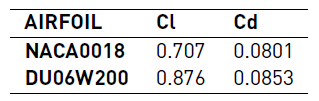
The DU06W200 produces 20% more lift coefficient than NACA0018, and its drag coefficient differs only by 6%. Therefore, the airfoil DU06W200 shows a better aerodynamic performance than the NACA0018 under the wind flow conditions of Chicamocha’s River.
4. Conclusions
Implementation of Vertical Axis Wind Turbines is feasible at Chicamocha’s river, where average wind speed is 7 [m/s] and average wind power density is 485 [W/m 2].
The “simpleFoam” solver is validated by using the Spalart-Allmaras fv3 turbulence model by its accurate results with a difference of 12% in comparison with experimental tests from literature.
The airfoil NACA0018 shows its higher performance at an angle of attack of 10° where the lift and drag coefficients ratio has the greatest value: 10.3 approximately
The new airfoil DU06W200 presented these results:
-Its lift coefficient increase 20% with the same drag loses as the NACA0018 airfoil at Chicamocha’s river wind speed.
-Lift coefficients for the DU06W200 airfoil at Reynolds numbers between 2 x 10⁵ and 3.4 x 10⁴ are 23% greater than the NACA0018 ones.
-Therefore, the DU06W200 airfoil shows a better aerodynamic efficiency for vertical axis wind turbines’ blades under wind properties of Chicamocha’s canyon.
5. Future work
The wind energy potential at Chicamocha’s canyon should include measurements during night time. In addition, the incidence of wingtip vortex on the finite wings should be calculated as well as the influence of the three airfoils distribution under unsteady simulations. Finaly, the geometry of the troposkein shape for the total wing design should be compared with a straight blade design.

