2.1 Characteristics of the study area

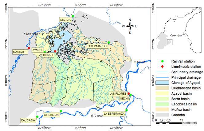
Ayapel Cienaga is located in the department of Córdoba in Colombia [Figure 1]. It is part of the macrosystem of wetlands and floodplains known as the Mojana region [⁷]. The floodplain basin has a total area of 1,504 km², divided in five catchments (Quebradona: 262.14 km² Cienaga: 112.77 km² Barro:515.62 km² Escobillas:146.02 km² Muñoz: 385.82 km²), with altitudinal variations between 20 and 150 masl. This floodplain is considered an important aquifer and reservoir of the alluvial plain of the San Jorge River [²], and has a landscape of permanent shallow wetlands with mean depths close to 6 m [⁸].

Figure 1 Ayapel Cienaga and basin location 

2.2 Hydrology of the Ayapel basin

We characterize the monthly hydrology of Ayapel with spatial spline interpolations using Arcgis, employing records from one principal (Ayapel, 1969-2015), six pluviometric (Cecilia, Los Pájaros, La Esperanza, Nechí, La Ilusión, and Caucasia from 1969 to 2015), and three limnimetric stations (Marralú, Beirut and Las Flores, 1974 to 2012) from IDEAM [Figure 1] [⁹].

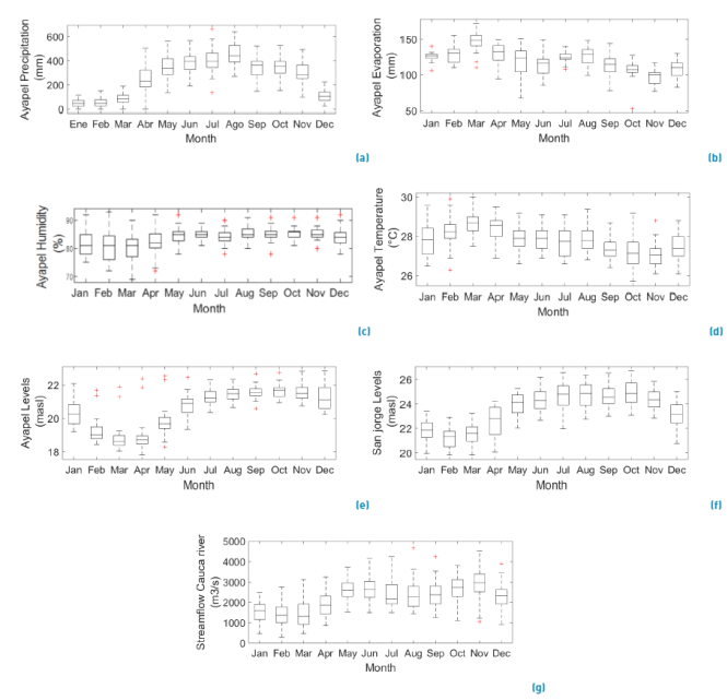
Figure 2 summarizes the multi-year monthly distribution of evaporation, precipitation, relative humidity and temperature over Ayapel. Evaporation varies between 90 mm and 150 mm. Precipitation is unimodal with a wet period from May to October and a dry period from December to March. The relative humidity is high, with average values between 80% and 90%. Temperature also presents a unimodal behavior inverse to precipitation, with a narrow variation between 26 °C and 30 °C. Ayapel flood pulse is slightly asynchronic with precipitation, exhibiting low levels between February and April and high levels between August and November. There are two transitional months (May and November), known as the rise and fall respectively, which benefit both agricultural activities and fish migration. We gather the limnimetric data (1985 to 2012) from the Beirut station, located in the southwestern part of the Cienaga.

Levels of the San Jorge River are synchronic with those of Ayapel. This river actually controls the outflows of the Cienaga to the north. The river monthly levels oscillate between 18 and 22 masl, with lows during the dry season (between November and April) and highs during the wet season until October. We obtained the San Jorge River levels, corresponding to the years 1985-2013, from the IDEAM limnimetric station in Marralú. Monthly discharges of the Cauca River in the area are similar to those of the Cienaga and the San Jorge River [Figure 8]. Lower flows occur in the first quarter of the year, while higher flows occur in June and November. Since the 1980’s, several levees (i.e., the Santa Ana and Nuevo Mundo) line the Cauca River along the southern reach of Ayapel, reducing the likelihood of floodings towards the Cienaga only to extreme events and levee failures, such as the one occurred in 2010.

Figure 2 Hydrologic and limnimetric information in the study zone: a)Precipitation, b)Evaporation, c)Relative humidity, d)Temperature, e)Ayapel level, f)Levels of the San Jorge river monthly and g)Streamflow of the Cauca river 

2.3 Relationship between hydrology and global climate indices

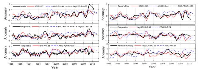
To understand how global climate relates to the hydrology of the floodplain, we correlate rainfall, temperature and levels with the most important climatic indexes for the region: The Pacific Decadal Oscillation (PDO), the Southern Oscillation index (SOI) and the Atlantic Multidecadal Oscillation index (AMO), obtained from NOAA. We compare 12-month moving averages of the anomalies during the period 1985 to 2012.

Figure 3 shows the anomalies of different global climate indices related to climate variables in Ayapel. The AMO, negative PDO phase (negPDO) and SOI indices positively correlate with the levels (especially SOI and levels, R = 0.71). The response to the 97-98 El Niño (one of the strongest in history) [¹⁰] is clear both in the levels and precipitation (0.57). Levels show the same behavior during a series of events of moderate La Niña years (98-99, 99-00, 07-08 and 10-11). Important ENSO and PDO relationships have also been found in other lakes in Colombia [¹¹]. When analyzing the temperature anomaly with the SOI and the PDO-AMO combination, we obtained a correlation R=0.38. The positive phases of AMO and PDO relate to conditions of high temperatures in the floodplain.

The Cauca River flow has the highest correlation with SOI (0.69), and lower with AMO and AMO-PDO combination (0.44 and 0.53 respectively). Evaporation shows its higher correlation with the negative phase of SOI (R=0.35), although the extreme values in this oscillation do not directly influence this variable. The relative humidity of the Cienaga showed a better correlation with the AMO oscillation (R=0.31) than with SOI.

Figure 3 12-month moving averages of levels, temperature, precipitation, Cauca River flow, evaporation and relative humidity related with the SOI, AMO and PDO indices 

2.4 Projected climate scenarios

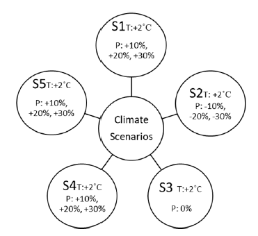
We evaluate the critical conditions in the Cienaga through five scenarios, using an increment of 2˚C in temperature in all of them and several conditions for precipitation [Figure 4]. Scenario 1 (S1) represents an increase in precipitation average. Scenario 2 (S2) represents a decrease in precipitation average. Scenario 3 (S3) represents a normal condition, with no variation in precipitation average and variance. Scenario 4 (S4) represents an increase in precipitation variance. Finally, Scenario 5 (S5) represents an increase in wet months and a decrease in dry months. In addition, each scenario has an increment or decrement (10%, 20% and 30%), based on different future projections.

Figure 4 Climate scenarios for Ayapel S1, S2: mean change S3: no change, S4: extremes change S5: variance change 

2.5 Fish dynamics

There is an important relationship between fish population, seasonal catches and wetland levels. Levels in the Cauca River, for instance, have been linked to human activities, in particular the capture of a fish of commercial importance called Pyaractus brachypomus, commonly known as "cachama blanca" [¹²]. We considered bocachico (Prochilodus magdalenae), which has the highest commercial value in Ayapel [¹³], as a representative species to study fish population dynamics in Ayapel. We established a directly proportional relationship between levels and population for bocachico fish in the Cienaga.

2.6 Mining

Most gold mining activities in Colombia are underregulated and do not have proper environmental permits [¹⁴]. That is the case of Ayapel, where mercury is used to extract gold, posing danger to the environment, especially to aquatic organisms and through them to humans [⁴]. This metal has become a polluting substance due to its overuse, mainly in gold mining activities, during the stage of amalgamation of gold. In aquatic macrophytes, for example, concentrations of mercury above 0.005 mg/l could affect the skin in humans and in plants can be metabolically absorbed by subtracting chlorophyll [¹⁵].

The amount of mercury that could reach the floodplain depends on the relationship between the mercury contribution and the mining production activities (1 Au : 6.1Hg) [¹⁶]. For instance, during 1996, about 108 tons of mercury were used to benefit 17.7 tons of gold in the Magdalena-Cauca basin, 50% of which is present in the water and 35% is emitted into the atmosphere [¹⁷].

2.7 Model structure

According to the previous description of the study site, we integrate three main balances in our model: 1) Hydrologic balance, 2) Fish population-catch balance, and 3) Mercury mass balance. A description of each follows.

Hydrological component

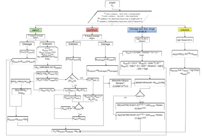
We estimate the monthly water balance in Ayapel from the inflows and outflows derived from precipitation, evapotranspiration, infiltration, runoff and stream and subsurface flows through a two-tank model applied over each of the five watersheds in the Cienaga. Water enters as precipitation in the first tank and leave subsequently in three fractions: evapotranspiration, direct runoff (established by means of a rainfall-runoff coefficient), and as seepage through the second tank that controls the amount of water that comes out as subsurface flow each month. The inflow to the Cienaga is the combination of runoff and subsurface flow. Figure 5 shows a flow diagram of inputs and outputs for the calculation of the monthly water balance of the Ayapel Cienaga. The balance has four main flow components: inputs, outputs, Ayapel and San Jorge levels and the Cauca River flows. The San Jorge River controls the outflow from the Cienaga to the north, whereas the Cauca River floods the Cienaga due to levee breaks.

Figure 5 Flow chart of hydrologic balance in Ayapel with connections using a two-tank model 

Precipitation: We projected precipitation (P) in scenarios S1 to S4, using a stochastic model with independent trend in the mean and the variance and considering the ENSO effect as a dummy variable. We used historical records of rainfall available from IDEAM for the period 1969-2012 [Figure 6], following the Equation (1)

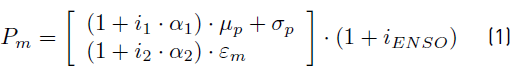
where P _m = projected precipitation; i ₁ = mean increase; mp: projecting month; α₁, α₂ = 1/mp = increase coefficient of mean (α₁) and/or variance (α₂); µ _p = Monthly precipitation mean; σ _p = monthly standard deviation; i ₂ = variance increase; Ɛ _m = random error N (0,1); i_ENSO= ENSO index (Niño or Niña).

The i_ENSO value depends on a z function, given by: La Niña= 0<z<0.2; Normal= 0.3 < z < 0.7; El Niño = 0.8 < z < 1.0. For La Niña years i_ENSO = (0.2+ z), for El Niño years i_ENSO = (0.8 - z) and for "normal" years i_ENSO = 0; i_ENSO allows the ENSO influence to be calculate on precipitation through a random function N (0,1) with a variation between (-0.2 and 0.2). The index ranges are given by the intensity of the climate phenomenon where ± 0.5 is the highest value giving way to El Niño or La Niña. Scenario 5 includes extreme variations over σ _p in wet and dry months given by (2):

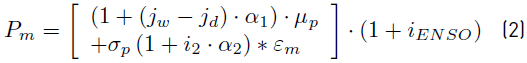
where j _w = Trend in average rainfall wet months [0 0 0 1 1 1 1 1 1 1 1 0]; j _d = Trend in average rainfall dry months [1 1 1 0 0 0 0 0 0 0 0 1].

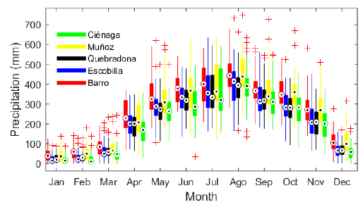
Figure 6 Multiyear monthly distribution of precipitation for each of the sub-basins contributing to the Ayapel Cienaga 

Temperature: We analyze temperature (T) with an autoregressive moving average model ARMA (1, 1), adjusted to historical series available for the period 1969 to 2015. Afterwards, we generated series with a Monte Carlo approach, using the Equation (3)

where T _t+1 = temperature projected at month t+1; T _t = temperature at month t; µ_T= mean monthly temperature; Ɛ= random term N (0, 1); α, β= model coefficients; ∆µ _T = projected average monthly increase of the variable.

Evapotranspiration: We estimate the evapotranspiration (ET) as a weighted average of two methods: Blaney-Criddle (ET _BC ), which use the temperature and a coefficient that depends on the type of vegetation, and Romanenko (ET _R ) [¹⁸]. The Equation (4) of Blaney and Criddle to estimate evapotranspiration, converted to metric units, is as follows:

where k = coefficient of monthly consumptive use, p = total daily hours percentage in a period on total hours in a year, T = average temperature in °C.

Equation (5) shows Romanenko evaporation relates the average temperature and relative humidityas:

where T = average temperature (°C) and RH = relative humidity (%)

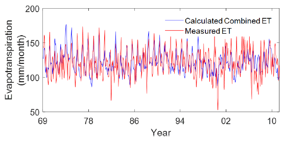
We normalize the values by subtracting the average and dividing by the standard deviation of the same series for each method. After assigning a weight to each series, we add the actual average (µ _er ) and multiply by the standard deviation of the measured ET(σ _er ). Figure 7 compares the measured ET with the generated for the historical period (6).

Figure 7 Comparison between measured and calculated combined evapotranspiration 

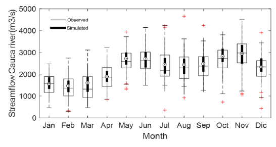
Cauca River flows: We calculate discharges from the Cauca River using an ARMA (1,1) equation similar to 3 with information of Las Flores station of IDEAM between 1974 and 2012, as shown in Figure 8. We generate random series with a Monte Carlo procedure to calculate correlation coefficients between observed and simulated data. We chose for the analysis the series that presented the highest correlation value.

Figure 8 Monthly diagram of the historic and simulated streamflows in the Cauca River 

The levees supposedly prevent the Cauca River from flooding the Cienaga. Nevertheless, the levees failed along the River’s left margin during 2010-2011, in three different sites: “Nuevo Mundo”, “Pedro Ignacio” and “Santa Anita” [¹⁹, ²⁰]. Our model quantifies, through conventional hydraulic relationships, the amount of water needed to overflow the Cienaga and reach the levels seen after the levee break of 2010. Specifically, we estimate the fraction of the total shedding that would actually reach the Cienaga water mirror, taking as inputs the difference between the Cauca River and the Cienaga levels. We model the breaks as a single event of lateral discharges towards the Cienaga.

Fish balance component

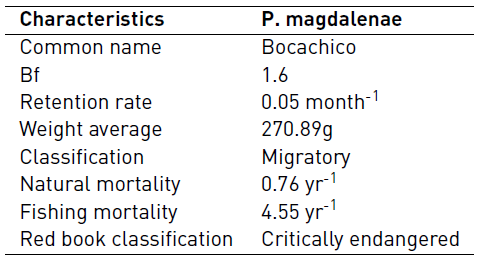
The bocachico monthly balance model [Figure 9], which considers historical extractions and those recorded after the Cauca River flooding in 2010, is based on the dynamics of fish populations established by FAO (7), that relates the death of fish due to two factors: a natural death rate in the population (M) and the fishing catch (F) [²¹].

Figure 9 Flow chart of bocachico population balance in Ayapel 

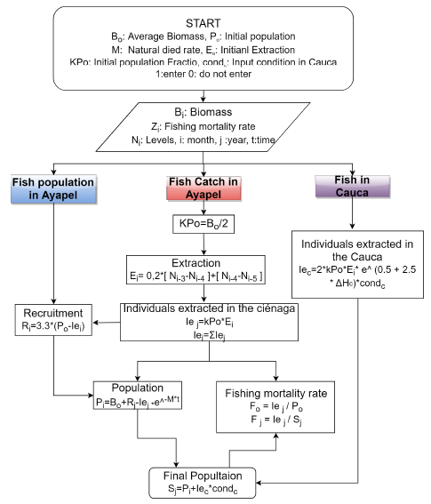
Table 1 shows general characteristics of bocachico (P. magdalenae) used in the fish balance model

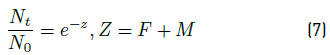
Where, t = time in months; N₀ = initial population (individuals); N_t = number of individuals in t; F = fishing-catch coefficient (1/month); M = natural death coefficient (1/ month); Z = total deaths coefficient.

The monthly balance is adequate to relate the birth, death and catch rates recorded for the bocachico in the area.

Table 1 General characteristics of P. magdalenae [²²]  

Mercury mass balance component

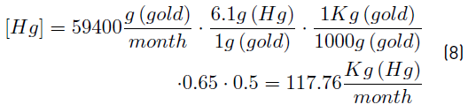
The Colombian mining information system provides monthly data of the actual gold production in Ayapel for the period 2001-2014 [²³]. With this information, we estimate the loads of mercury that could enter the Cienaga as a function of a mercury to gold extraction ratio. For instance, an average monthly production of 59.4 kg of gold may produce a load of mercury given by Equation (8):

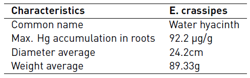
Mercury in Eichhornia crassipes (Water Hyacinth): E. crassipes is an aquatic plant present in Ayapel, whose coverage relates to the Cienaga’s annual pulse. The species adapts well to the environment due to its capacity for metal depuration, nutrients assimilation and spatial mobility [²⁴] [Table 2].

Table 2 General Characteristics of E. Crassipes 

Mercury in Prochilodus magdalenae (Bocachico): For the mercury balance in the P. Magdalenae, we used the study conducted by [²⁵], which includes: the concentration of mercury in the water, a retention rate and a bioconcentration factor (Bf). The latter describes how much Hg concentration is transferred to biological tissues using the Equation (9) [²⁶].

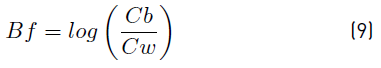
where Bf= Bioconcentration factor in Bocachico; Cb = mercury in tissues (2,080); Cw= mercury concentration in an abiotic component (water) (0.055ppm).

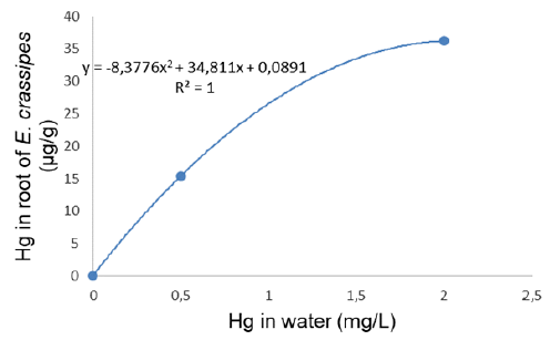
With the information reported by [²⁷], we adjusts a polynomic curve to calculate the Hg absorption equation (AbsEc) as a function of the Hg concentration in water [Figure 10 and Table 3].

Figure 10 Relation between Hgw and Hgroot after 30 days. Polynomic fit 

Table 3 Relation between Hg in water and Hg concentration Hg in roots [²⁷] 

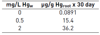
The flow diagram of Figure 11 shows the calculations of the monthly mercury balance in the Cienaga, considering three concentration matrices: water, macrophytes and fish. For this balance we made the following assumptions:

• Gold production records come from artisanal mechanisms using mercury for their extraction [²³].

• Annual gold production (AuProd) records are divided by 12 to have the monthly production.

• 30% of the mercury that enters the Cienaga (HgProd), is transferred to the sediment.

• E. crassipes covers 30% of the water mirror, which is consistent with the maximum observed in the field at different times of the year.

• The Cienaga waters are fully mixed each month.

• The number of individuals of E. crassipes (IndEc) is fixed, according to the average area of the Cienaga (Ac = 70 km²).

• Mercury is absorbed first by macrophytes (E. crassipes) and the rest bioaccumulates in fish.

• The number of fish individuals is fixed (Indpez = 50,000).

Figure 11 Flow chart to estimate mercury concentration in water, macrophytes and fish in the Cienaga 

3.1 Hydrologic balance component

Calibration and validation

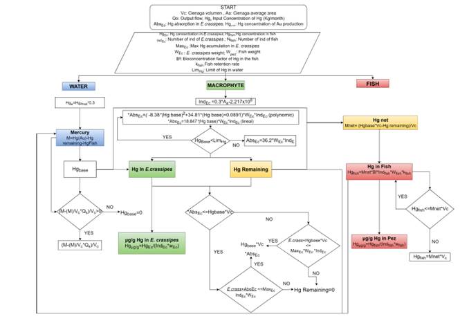
To calibrate and validate our model, we use bathymetric information registered by [²⁹] in 2004 and 2005. Figure 12 shows the topology of Ayapel, using functions which represent the variation of volume (lineal) and area (polynomic) with height. We use historical daily information during the period 1985 to 2010.

We calibrate our two-tank hydrologic model [Figure 5] and compare our flows with those simulated by [²⁸] in 2015. Table 4 shows the infiltration and runoff coefficients per catchment [²⁸].

Figure 12 a) Height vs Volume and b) Area vs Height in Ayapel [²⁸] 

Table 4 Coefficients used by sub basin in Ayapel 

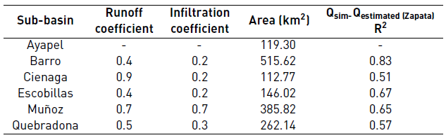
Our model allows quantifying, through conventional hydraulic relationships, the amount of water that could have entered the floodplain to reach historical levels, specifically the water fraction that would actually reach the floodplain waterpool. To simulate the condition observed in 2010, we considered the overflow over an equivalent single breaking site, located in “Nuevo Mundo”, using the Cauca flow projection with a lateral weir Equation (10) of the form:

where, Hc = Lateral discharge level of Cauca River (m), Q_c = Cauca estimate flow (m³/s), A =Measured flow average (m³/s), B = coefficient assumed by the landfill (1.5). H_base = heigh in the Cauca riverbed (25 m), Q_dam = Floodplain potential income stream (m³/s), Cd = coefficient (0.25), L_dam = overflow length (31 meters).

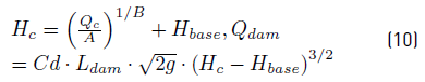
We simulated the series of levels (m), volume (millions of m³) and area (km²) and compared with the historical real series. Volume reaches a correlation of 0.86. Actual level data, obtained from the Beirut station of IDEAM from 1985 to November 2013, reaches a correlation of 0.87. Finally, the area has a correlation value of 0.85. The square corresponds to the imbalance in each of the three series due to levee breakings on the Cauca River. Figure 13 shows the actual levels due to the entrance of the Cauca occurred in 2010, compared to the expected levels under no break condition. In this way, our model allows the evaluation of the expected hydrologic conditions under no levee break. According to the model, the water discharges required by the floodplain to reach the levels observed in the period of the levee break were between 10 m³/s and 70 m³/s (this flow represents only the fraction of the total derivation required to maintain the floodplain level of the water mirror at recorded levels).

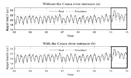
Figure 13 Observed and simulated levels (a) with and (b) without the estimated Cauca River entrance (period 1985-2015) 

Since the time we developed our model, a major controversial hydroelectric project over the Cauca River was built upstream Ayapel and has been in operation since 2019 [³⁰]. This project changed the normal dynamics of the river and therefore, it will likely influence Ayapel levels in the future.

Results of scenarios

With the model, we project the Cienaga levels for the five proposed scenarios under the conditions of variation of precipitation of 10%, 20% and 30%. For this, we calculate the difference in meters between the monthly historical average level (zero value in the graphs) and the monthly average of the projections (between -1.5 and 2.0).

Scenarios S1 and S2 show significant level variations, which increase or decrease proportionally to the increase or decrease in the defined percentages. In Figure 14, S2 makes more evident the decrease of averages in the rainy months (April to November), which imply that drought conditions may affect agriculture and fish migration. As expected, the scenario S3, which represents the projection of current conditions, does not show significant differences with the historical average.

Increase in variance (S4) does not seem to have a decisive influence on these differences, especially from June to December, when high rainfall occurs in the Cienaga. For S5, which establishes a variation in the extreme values of rainfall, the projected averages surpass the historical average in most months, which indicates that the levels maintain an equilibrium despite the water deficit in dry months, possibly due to the connections with flows and streams that enter the Cienaga. Hence, the Cienaga is able to buffer the extreme conditions under these two scenarios. The extreme values correspond to those upper and lower monthly peaks in the levels.

According to projections established by [³¹] for the region, it is expected a reduction in rainfall by the year 2040. In spite of this, given the historical rising trend in levels, and according to these changes in monthly averages, the S1 (10%) can be considered the most likely scenario, and S2 (-30%), would be a pessimistic scenario. While the optimistic scenario is the S4, where the differences in the historical averages would not undergo significant changes in a projection until the year 2045.

Figure 14 Monthly difference between projected averages per scenario and the historical average in Ayapel levels anomalies with variations in rainfall mean of 10%, 20% and 30% in scenarios, maximum and minimum values (+) S5 S4 S3 S2 S1  

3.2 Fish balance component

For S3 (“historical”), Figure 15 shows the estimated bocachico catch bar, the expected fish population after the balance and the catch reported from 2005 to 2015 by Colombian fishing Statistic service (SEPEC) and the Agricultural Statistic System (SEA) [³²]. The population responds to changes by catch. Population in terms of biomass varies in the historical period from 191,700 kg / year in 1990 to 235,100 kg/year in 2000. With the levee failure, the extractions exceeded the limit over 400,000 kg in the most critical year (2011), which can be interpreted as a piston flow that diverted a population of bocachico from the Cauca River to the floodplain, which was not part of the normal balance. After this event, the estimated catch and populations went to normal and the system recovered its capacity with a negative loop. The concept of a loop is very useful because it allows us to start from the structure of the system to analyze and reach its dynamic behavior [³³]. To say that the system has a negative loop is synonymous with finding the dynamic balance in the population.

Figure 15 Bocachico biomass vs catch for the period 1985-2044, including real data catch, for S3 

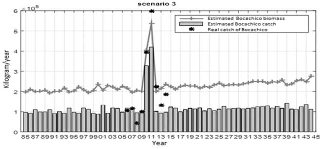
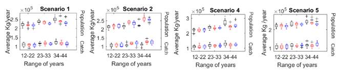
Figure 16 shows the projected bocachico population in term of biomass (Population) and the projected bocachico catch (Catch) for the scenarios of precipitation (±10%, ±20% and ±30%) through the projected period of 2012 to 2044, in a range of 11 years.

For S1, +10% corresponds to high values in the bocachico population around the 250,000 Kg/year at the end of the period (2034-2044). The condition +20% and +30% show a small increment in population. The extractions remain similar during all the period. Despite a slight increase in the trend, as the rainfall increases, the population percentages appear to be stable. Also, in this scenario, the relation between rain percentage change and fish population is inversely proportional. For S2, a significant change in trends of -20% and -30% is seen in both the population and the catch. The highest population value occurred in the range of year 2034-2044 in -20% where the population exceeded the 250,000 kg/year. The rain percentage is directly proportional to the population and inversely proportional with the catch. The catch does not have significant variation between the range years but maintain the same behavior like the population. In S4, which represents changes in the variance, the behavior between both average projected population and average projected catch presented not significant change. The years ranges 12-22 and 23-33 have similar average for each percent for the population and catch. Only in the range between the years 34-44 the average population biomass exceeds the 250,000 kg/g with the condition of 10% associated to an increment in the catch. In S5, there are not significant differences in the catch during the different periods. The population trend seems not to have been pronounced significantly, only the last one (34-44) appear to increase in the three conditions. Thus, population is able to maintain equilibrium.

Figure 16 Population vs. catch of P. magdalenae by the range of projections 2012-2044 under variability scenarios S1, S2, S4, S5 with the variation in average, variance and extremes ±10% ±20% ±30% 

3.3 Mercury mass balance component

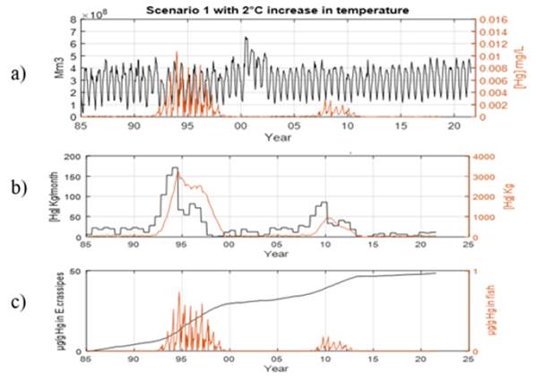
Starting from the initial conditions mentioned above and under the assumption that macrophytes absorb mercury in water before fish, we calculate the accumulations for the period 1985-2045 shown in Figure 17 for scenario 1.

This model is a conservative approach to estimate the concentration of mercury (coming from environmentally inappropriate gold mining in the Cienaga) not only in water but also in two important ecological compartments such as fish and macrophytes. We consider the Cienaga as a fully mixed system. The monthly concentration of mercury (mg/L) in the Cienaga relates inversely to the mixing volume of water (low levels and monthly inputs increase concentration). These changes in concentration can affect the levels of bioaccumulation in the Cienaga [⁶].

Let us consider, for instance, the 1985 production with an income of mercury to the Cienaga of 5.8 KgHg/month. The mercury accumulated in E. crassipes begins to increase but there is no incorporation in the fish. Only until the year 1997 does a bioaccumulation appear on the part of the fish of the order of 1.43x10^-3 μgHg/g and in E. crassipes of 5.8 μgHg/g with an income of 100 KgHg/month. In the year 2001, the polynomial model reaches an amount of mercury deposited that exceeds 3000 KgHg/month, corresponding to the highest peaks in the whole simulation.

As of 2010, when production begins to fall, E. crasspies continues to incorporate mercury, but more gently tending to stabilize. This makes the incorporation into the fish almost null until later in both proposed models, since the macrophytes are able to accumulate all the available mercury. Then, when there is a projected increase due to an impact on the exploitation of gold, the macrophytes take advantage of this income again with a concentration of 34.5 μgHg/g. The accumulation in fish, on the other hand, would be lower.

Figure 17 a) Monthly variations of water volume and mercury concentration in the Cienaga; b) amount of mercury that may arrive in the Cienaga; and c) estimated concentration of mercury in macrophytes and fish 

3.4 Model limitations

Our model is an attempt to integrate several compartments of relevance in the description of the Ayapel Cienaga. The hydrologic model, for instance, works on the catchment scale, since we determine that the Cienaga responds mainly to the local rainfall and only in extreme cases to the dynamics of the Cauca River. This scale is also adequate to integrate the fish dynamics that respond synchronically to the Cienaga flood pulse. The incorporation of mercury from local mining practices can also be described in monthly intervals, given the bioaccumulation rates in the native macrophytes and fish, and considering the conservative nature of the pollutant once incorporated to water and sediments. In this regard, our model describes an aggregated, conservative approach, to these balances. The model does not provide detailed descriptions of groundwater recharge, or inner hydrodynamics of the Cienaga, which require information on more refined scales. The model does not consider the impact of increasing temperatures on the metabolism of fish (reproduction and mortality rates), which may also decrease the expectations of fish population in the proposed scenarios. Furthermore, it is important to clarify that our model does not consider the impact of the Hidroituango dam on fish populations downstream, or in the likelihood of extreme floods, which is still a subject of discussion and may alter considerably the results projected in our scenarios. Nevertheless, the conceptual framework and outcomes of this model may serve as a baseline for further models at other scales, and as an aid for decision-makers and academicians concerned by the environmental management and protection of the Cienaga.