


 Inglês (pdf)
 Artigo em XML
 Referências do artigo
 Enviar este artigo por email
 Citado por SciELO
  Citado por Google
  Similares em
SciELO
Similares em
SciELO  Similares em Google
 Permalink
1. Introduction
The use of bicycles as public transportation has increased in the world since the 1960s. Cities around the world are developing more accessible bicycle sharing systems (BSS) in order to enhance the use of this transportation mode for commuting and/or physical activity. There are many expected benefits of cycling as public transportation: the reduction of fossil fuel consumption, the increase of physical activity, and the reduction of congestion in the cities [1-3]. In order to provide suitable infrastructure for cycling, governments need to invest in bicycle lanes, stations, comfort, continuity of roads and promote the integration of the BSS with traditional transportation paying schemes, among others. Policy makers and city planners should be aware that this kind of investment must be in tune with the growing use of each BSS [2, 4, 5].
The selection of the bicycle as a transportation mode will depend on factors such as the age of the user, gender, safety, lane infrastructure, health benefits of cycling, and health risks associated with air quality on the road [6-8]. Users of BSS and walkers are exposed to harmful pollutants as they are in direct contact with mobile sources [9-11]; therefore, they might lose all the health benefits from the outdoor activities [12]. Concentrations of pollutants on roads are directly influenced by road congestion and the overall atmospheric conditions in the surroundings [13-15], and according to recent research, the availability of real-time pollution information, provided by sensors and smartphone applications, may influence the frequent user on the decision of taking out a bicycle [16, 17]. Particulate matter measurements techniques are mainly divided in two, the measurement of particle concentration and the measurement of particle size [18]. Particle size measurements are important as they give information of the dynamics of the particle and persistence in the atmosphere [19]. Concentrations of a defined size of particle are important for the definition of emission limits and permitted concentration in order to guarantee safety [20, 21].
According to the World Health Organization (WHO), Medellin is one of the most polluted cities in Latin America, reaching average concentrations of fine inhalable particles with diameters of 2.5 micrometers or smaller (PM2.5) of around 26.7 μg/m3 [22]. Air pollution in the city has a daily cycle with two peak hours, one early in the morning and a second one in the afternoon, both related to peaks in traffic and industrial production. Air pollution is affected by two processes, namely the temperature inversion in the atmosphere of the valley where Medellin is located, and the atmospheric stabilization during the dry-to-wet (March-October) season transition [23, 24]. Due to this well-known issue of air pollution, the city has invested in air pollution management by increasing the number of monitoring stations all over the metropolitan area and by promoting public policy to improve transportation and the quality of fossil fuels in the country [25] (www.siata.gov.co).
The Medellin metropolitan area, in Colombia, has incorporated the goal of promoting bicycles as sustainable urban transportation in its urban development policies. The region defined in 2015 its most recent bicycle public policy, including concrete plans for bicycle infrastructure expansion, which is expected to promote bicycle demand, projecting it to be up to 10% of the total trips made in the city [26]. Additionally, the BSS in the region, known as EnCicla (www.encicla.gov.co), was implemented in 2010 to promote sustainable mobility. EnCicla started its operation with six stations and 105 bicycles and currently has 51 stations, including 32 automatic stations and 19 manual operations, and more than 1,300 bicycles and approximately 92,000 active users. According to EnCicla, the system accounts for 30% of bicyclists in the city with user ages ranging from 16-75 years.
Air pollution is then an important issue for the cyclists and pedestrians in Medellin, and the monitoring of pollutants on a route may be a key factor for decision-making in areas such as the improvement of biking infrastructure, the development of early warning systems, or the proposal of design parameters for new routes to be constructed. Here, we present the first effort in the city to study the concentrations and potential exposure of cyclists to PM2.5 in the EnCicla system incorporating seasonal and diurnal variations. The work is organized as follows: Section 2 outlines the methodological approach and includes the definition of the study area, how sensors are used and validated, the monitoring protocols, the calculation of the potential average daily dose, and the detection of hotspots on the route. Section 3 provides the results found and the discussion. And in Section 4, concluding remarks are presented.
2.Material and methods
2.1 Study area
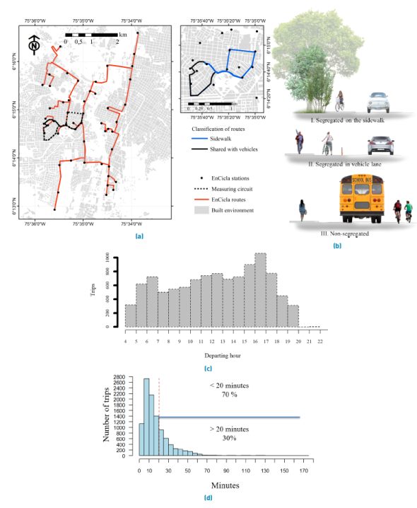
EnCicla is a BSS with 51 stations and more than 35 km of routes that are divided into three types of lanes [Figure 1a and 1b): i) segregated on the sidewalk (25.3 km), ii) segregated in a vehicle lane, separated by vertical elements (9.5 km), and iii) non-segregated, where the bicycle shares the lane with automobiles (0.2 km). According to the origin/destination information of the BSS, there are three peak periods of use, a morning interval from 06:00 to 07:00 hours, another in the middle of the day from 12:00 to 14:00 hours, and a third one in the afternoon from 16:00 to 17:00 hours [Figure 1c). We defined a 5-km circuit within the routes of the system in order to monitor the PM2.5 concentrations. The circuit is located in a relatively flat portion of the city where the mean altitudinal difference between stations is no more than 35 m in 2 km (gradient < 2%), thus reducing the influence of gradient in the efficiency of vehicles and facilitating the measuring procedure for bicyclists. The circuit also goes along heavy-traffic roads, intermediate-traffic roads and residential roads [Figure 1a).
2.2 Use of sensors
Sensors are a suitable technology for monitoring and analyzing air pollution concentrations, with proven accuracy and practicality for: the configuration of air pollution monitoring networks [27], real-time analysis on a route when installed in cars [28], and also for measuring when installed on bicycles [29-31]. In particular, the AirBeam sensor has been on the market for several years and it has been in continuous development since its introduction in 2014 (http://aircasting.org/). This is low-cost, easy-to-use equipment used in citizen participatory research that offers a suitable tool for the monitoring of air pollution [32-34]. The AirBeam is equipped with a Shinyei PPD60PV particle sensor [35] that extracts air through a detection chamber in which the light comes from an LED bulb scattering particles in the air stream. This scattering of light is recorded by a detector and converted into a measure that estimates the number of particles in the air. These measurements are reported approximately once per second via Bluetooth to the Android application AirCasting [36]. The precision of the device was tested with three different pollutant sources, showing coefficients of variation of less than 10% when compared with measurements made with professional particle-sizing and analysis equipment [37]. Also, the sensor has a good performance for humid environments, making it a good option for measuring in a humid tropical setting such as Medellin [38].
2.3 Validation of the sensor used
We validated the use of AirBeam sensor for the local conditions as recommended by [37]. The validation consisted of calculating a Pearson Correlation Coefficient [39] using 1,000 bootstrapping replicates in order to construct a 95% interval due to the [40] between the AirBeam measurements and the measurements produced by the air-quality stations installed by the local environmental agency in the Sistema de Alerta Temprana de Medellín y del Valle de Aburrá (SIATA - https://siata.gov.co/). This network has 18 calibrated stations used to monitor PM2.5 concentrations in the region. Aggregated data can be accessed after a quality control process at www.siata.gov.co. In a second stage of validation, we compared the general daily cycle features (hourly peaks in concentration) of our measurements with the atmospheric backscattering data produced by one of the ceilometers [41] near the monitoring route. Ceilometers in the SIATA network are used to measure the vertical profile of the atmosphere; these instruments are simplified Lidar systems, which operate in the near-infrared wavelength range, giving information about the energy that is backscattered by particles in the atmosphere. Atmospheric backscattering can be used as a proxy for the concentration of aerosols and particles in the atmosphere [42, 43]; therefore, it may indicate if the general performance of the sensor is responding to the presence of pollutants in the atmosphere.
2.4 Monitoring protocol
A successful measurement consisted of a complete circuit within the time lapse from one hour to the next (e.g. 06:00 to 07:00), and complete daily monitoring comprised 13 measures from 06:00 to 18:00 hours, in order to include the peak activity on the BSS [Figure 1c). The monitoring system includes: i) AirBeam connected to its mobile application (AirCasting) previously installed in a smart phone, providing measures of PM2.5 and global positioning system (GPS) coordinates each second, and ii) a cyclist who carries the sensor and the mobile phone whilst cycling around the circuit. Each monitoring circuit was carried out during meteorological dry conditions for two reasons: i) BSS users decrease significantly during episodes of rain, and ii) precipitation may alter drastically the concentrations of PM2.5 in the atmosphere.
2.5 Potential average daily dose
Following the EPA Exposure Factors Handbook [44] and the work of [45], we computed the potential average daily dose (PADD) of bicycle users riding twice a day ( one round trip) with an average trip duration of 20 min [Figure 1d). PADD is defined Equation (1):
where C is the concentration of PM2.5 (µg/m3), IR is the intake rate (m3/d), ED is the exposure duration (h/d) during a 1-year period, and BW is the body weight (kg) of the cyclist. IR is assumed according to the average traveling speed during the monitoring protocols based on inhalation rate values recommended by the International Commission on Radiological Protection (ICRP). For male adults, IR is 1.5 m3/d, and for adult females it is 1.25 m3/d for light effort. In the case of moderate/strong effort, IR for male adults is 3.00 m3/d, and for female adults it is 2.70 m3/d [45]. PADD is a key measure to understand the actual amount of pollutant that reaches the tissues of the exposed individual [46], thus the monitoring of air quality is necessary but not enough to study the potential threat that pollution may have on active individuals as the bicyclists.
2.6 Detection of hotspots
We selected the hourly routes with a mean concentration of PM2.5 equal to or higher than 25 μg/m3. This is considered as a control value because it is the condition of mean concentrations in the city reported by the WHO, and therefore we assume that higher values are due to unusual conditions. After detecting those routes with a mean value above the control and use the Shapiro-Wilk test [47] to identify if the hourly data is normally distributed, we defined a threshold for the identification of hotspots as locations measured on the route reaching concentrations higher than three standard deviations above the mean value (both calculated with the measuring records of the selected route). This threshold represents persistent concentrations above the environmental conditions that may be occurring due to the configuration of the route (e.g. traffic lights, interaction with vehicles or obstacles to the dispersion of pollutants). After detecting hotspots, we compare the concentration and daily cycle of the concentrations measured on the hotspots and the route for a detailed analysis.
3. Results
3.1 Validation of the sensor
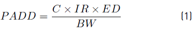
During 50 hours, we measured close to one of the SIATA stations (UNAL) in an outdoors non-controlled environment, as similar as possible to the conditions that we might find measuring on route. We used hourly average concentrations from the AirBeam sensor and hourly averaged concentrations reported by SIATA [Figure 2]. We found a Pearson correlation coefficient in the range of (0.81 - 0.94) with a 95% confidence that can be explained by the differences in the methodologies for measurement, we have to remember that stations rely on low-vol measurement equipment and filter weighting and sensors in light scattering. We found that the sensor has a root mean square error (RMSE) of 7.6 µg/m3 and a normalized RMSE (NRMSE) of 13%. This first result of validation shows that the sensor has fairly good representation of the concentrations near the station as found recently by [48] for outdoor studies.
We complement the validation with a qualitative comparison between measurement circuits and the vertical profiles of backscattering for three days: March 28, June 18 and June 28 2018 [Figure 3]. On March 28, during the season transition, PM2.5 concentrations were higher than 30 μg/m3 for most of the day, especially from 06:00 to 10:00 hours, while backscattering showed clouds around 1,500 m above the surface (red); there was high backscattering due to particles all day, but it was more intense from 00:00 to 12:00 hours [Figure 3b). On June 18, concentrations of PM2.5 were around 10 μg/m3, and the backscattering pattern was characterized by clouds higher than 3,000 m above the surface and low backscattering near the surface [Figure 3c). On June 28, we measured a peak PM2.5 concentration of 63 μg/m3 at 09:00 hours, and although the backscattering plot showed intermittency in the clouds around 1,500 m above the surface that may have led to more effective dispersion of pollutants, we observed high values for backscattering from 0 to 500 m above the surface that peaked around 09:00 to 10:00 hours and were abruptly reduced at 11:00 [Figure 3c) as measured in the circuit [Figure 3a).
As studied by [49], the vertical profiles of backscattering in Medellin during March are characterized by the presence of clouds in the early hours of the morning that configure the valley’s atmospheric boundary layer, around 1,500 m above the surface (red color in the backscattering plots in online Figure 3b and 3d), and the presence of high backscattering (light blue in online Figure 3b) below this level due to the concentration of aerosols in the lower atmosphere. These clouds starts to disappear around midday, giving pollutants a way to ascend toward the higher levels of the atmosphere. In conditions of a clear sky or clear atmosphere, less backscattering is presented (intense blue in Figure 3b to 3d). According to previous results, we are able to verify that the sensor used provides measurements on site that are consistent with the dynamics of the atmospheric concentrations of aerosols and particles in the region [Figure 3a compared to Figure 3b to 3d).
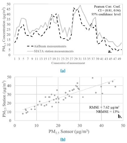
Figure 2 Comparison of measurements between the AirBeam sensor and the UNAL SIATA station. Time series of concentration during the 50 hours of measurement (a), Station and Sensor concentration scatter plot (b)
3.2 Monitoring protocol results
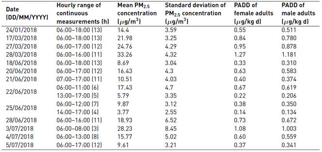
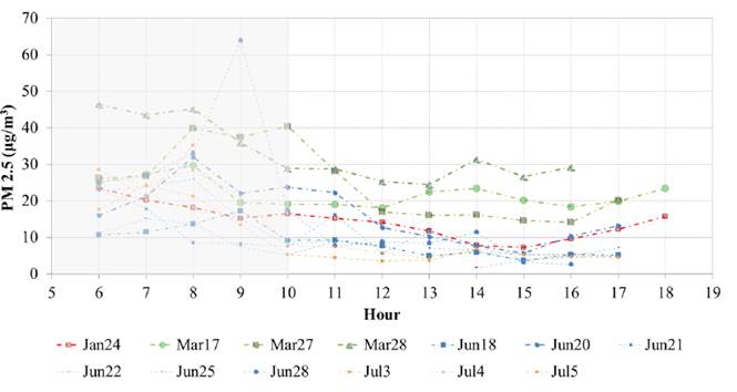
For 13 days, we completed 141 h of complete measuring circuits. The dates of the measurements were defined according to two criteria: i) days during the dry season when rain would not interfere with the measurements (February, June, and July); ii) days during the dry-wet transition when the atmospheric stability increases the concentrations of pollutants in the region (March). The average PM2.5 values in the hours measured during the days of monitoring are presented in Table 1. Mean values for reported days with more than 10 continuous hours of measurement in the dry season ranged between 9.6 and 18.9 μg/m3, while in March, during the season transition, concentrations ranged between 20 and 33 μg/m3. The daily cycle of concentrations shows that between 06:00 and 10:00 hours, concentrations are consistently higher than those in later hours (shaded region in Figure 4].
Concentrations of pollutants during the early morning in the region are related to the process of thermal inversion in the local atmosphere that makes the upward movement of pollutants difficult. This result shows how environmental conditions are the main driver of high pollutant concentrations in the region and therefore along the bicycle routes.
3.3 Potential average daily dose
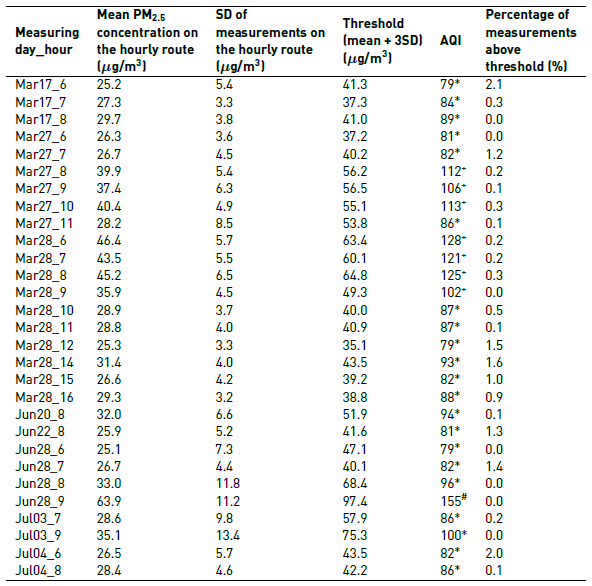
Daily cycles of concentrations reveal that in the early morning it is possible for mean values to reach up to 63 μg/m3 [Figure 4 and Table 2]. Those values may be considered as harmful for sensitive groups or even harmful for everybody according to the air quality index (AQI) calculation defined in the regional normativity [50]. The average time for each monitoring circuit is 40 min, resulting in an average speed of 6.7 m/s that we will consider as moderate to strong effort (IR for males 3.0 m3/d and for females 2.7 m3/d). PADD ranges between 0.13 and 1.18 μg/kg/d for males and from 0.14 to 1.27 μg/kg/d for females, showing that it is highly dependent on the season as it is doubled from January to March, and also can be increased by 30% if PM2.5 is averaged for morning hours or afternoon hours (see June monitoring dates in Table 1].
Table 1 Mean and standard deviation of the hourly ranges of measurement during each of the dates of measuring
3.4 Detection of hotspots
We identified 29 hourly measuring hotspots with mean PM2.5 concentrations above 25 μg/m3 (20% of the total hourly measurements). As expected, most of the hotspots were within the period, 06:00 to 10:00 hours, except for March 27 and 28, during the season transition (dry to wet) when the atmospheric stability maintains conditions unfavorable to pollutant dispersion. The persistent high concentrations on the route of about three standard deviations above the mean value are considered as hotspots, and in total do not reach more than 2.1% of the measurements in the selected hours; in some cases, there were no values higher than the threshold to identify any hotspot in the circuit (shaded in gray in Table 2]. After the theoretical identification of hotspots, we proceeded with identification of the hotspots on the route map [Figure 5] and on site. We made a photographic register of the physical configuration of the hotspots (Supplementary material).
Table 2 Hourly routes with mean concentrations higher than 25 μg/m3. AQI values are dimensionless and were calculated according to [50]; values marked with asterisks are in the range 51-100 and classified as moderate, values marked with a plus sign are in the range 101-150 and classified harmful for the health of sensitive groups, and values marked with a hashtag are in the range 151-200 and classified as harmful for health
Onsite inspection of hotspots permitted us to define two types, according to the built environment: i) canopy tunnel and ii) road intersection. The main characteristic of a canopy tunnel is the closure of high tree canopy over the cycling route. The road intersection type of hotspot corresponds to those places where cyclists needed to wait for more than 2 min in order to cross heavy-transportation roads. The factors identified that influence the concentration of pollutants at those intersections are that: i) the average speed of vehicles is reduced in order to stop for red lights and to start up after green lights; ii) the number of vehicles waiting for a green light increases the number of sources near the cyclist; iii) busy roads include heavy traffic such as buses and trucks.
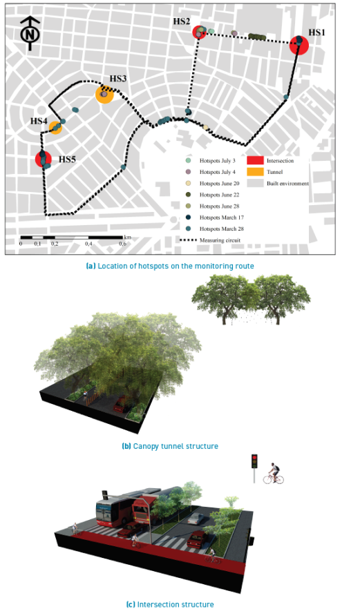
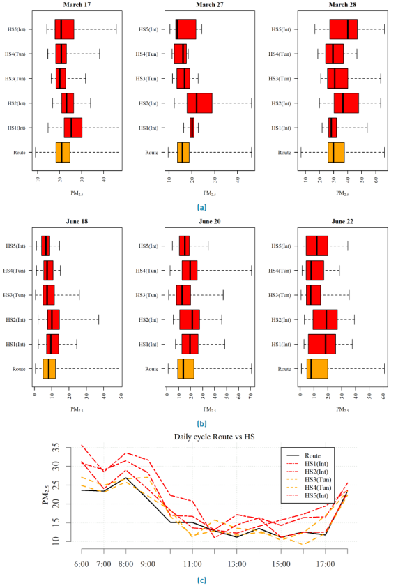
We selected 5 areas (HS1-HS5) representing intersections and canopy tunnel structures as the detected hotspots [Figure 5a). We compared the distribution of the concentrations measured in each of the HS areas along the route for six selected days using all the hourly measurements available, three in March and three in June. Mean concentrations in March are higher than those found in other months [Table 1 - section 3.2), these can be seen in the mean values for the complete route measurements and HS areas when comparing Figure 6a and Figure 6b. For the three days in March, we found that the third quantile values of HS2 and HS5 are consistently higher than those along the route; we can observe this for HS1 for March 17 and 27. HS3 and HS4 mean values are higher than values along the route for all days in March, and the third quantiles are higher than those along the route for March 28. This result shows that for March we can observe higher concentrations of PM2.5 on the selected hotspots. For June, we find that HS1 and HS2 have higher mean values and third quantiles when compared with values along the route. These results suggest that for high background concentrations like those found in March both canopy tunnels and intersections act as hotspots, while for lower background concentrations like those in June, only intersections present the hotspot characteristics. We can observe in the daily cycles at the HS areas that the concentrations during the day are consistently higher in the Intersections (HS1, HS2, and HS5) than those measured along the route or in canopy tunnels [Figure 6c).
4.Conclusions
According to our results, exposure to PM2.5 in the Medellin BSS is higher in the morning, between 06:00 and 10:00 hours. This is one of the periods with higher activity in the EnCicla system in terms of the number of travelers. In Medellin, universities start classes at 06:00, and most offices open at 08:00; therefore, journeys using bicycle made by students and people on their way to work are (negatively) affected because of the higher values for particle concentrations. Results show that in the dry-to-wet season transition, concentrations in the morning may be around values which are classified as harmful for sensitive groups of people (eg. children or elderly), therefore bicyclists should be aware of this situation if they are included in these groups and use effective protection such as masks [51, 52], as implemented in other countries such as The Netherlands and China. They should also make short journeys, combining their trips with the public transportation system with integrated BSS stations, to avoid extreme exposure. Including pollutant concentrations in the Equation when deciding for the bicycle as a mean of transportation may induce a decrease in the system demands during the season transition that should be included in the planning of new routes or bicycle acquisition.
PADD based on the daily exposure of cyclists shows that the intake of PM2.5 drastically changes by the season and by the hour in the day when they travel. According to the origin-destination data from EnCicla, journeys in the system are on average between 5 and 20 min. Exposure to the high concentrations of PM2.5 such as those found in the hotspots therefore may not be so harmful, since cycling only starts to be harmful after 120 min. in those environments with background concentrations between 44 and 150 μg/m3 [12]. Nevertheless, hotspots may represent harmful locations for other activities such as street vendors or traffic officers (police or other) or garden maintenance workers and pedestrians. Even though the hotspots were identified in a BSS-specific study, the results should open up the discussion about the impacts on health when choosing a particular route, and mode of transport, and hour in the day to travel.
Infrastructure should protect the user from direct contact with vehicles and the possibility of accidents, but in any case, it is a way of protecting from pollutants. Particular interventions in the infrastructure should be designed in order to achieve reductions of particle concentrations related to route configuration. Alternatives such as vegetation (Mejía-Echeverry et al., 2018), water sprinklers [53] or even electromagnetic capture must be further studied in order to develop new bicycle routes that protect the user not only from other vehicles but also from the traffic pollution.
Canopy tunnels are attractive to the user in bicycle lanes for two main reasons: i) an appealing landscape and ii) thermal comfort. Indeed, trees have the capacity to retain and absorb particulate matter produced by automobiles [54, 55], but the rates at which these particles are being produced is higher than the absorption capacity of the trees. Such canopy tunnel configurations were also identified as pollutant hotspots in a study of the expansion of the local bus rapid transit system in the city [56]. The physical structure of a canopy tunnel creates a blockage for the dispersion of pollutants in the atmosphere. It also causes lower temperatures at the ground surface than at the top of the canopy which also prevents pollutants from ascending, due to the effect of thermal inversion in the atmosphere. The option of strategic cuts in the canopy, so as to protect the ecological integrity of the routes and to ensure the vertical dispersal of particles, should be further studied.
Road intersections are designed to privilege automobile mobility. At many of the intersections detected as hotspots in this study, there was a high traffic of diesel buses and trucks which, in the region, do not yet reach Euro IV standard. At busy intersections preference is given to motor vehicles; therefore, the cyclist have to wait for up to three changes of vehicle red lights before they get to continue, which accounts for more than 2 min. of waiting. One way to tackle this problem may be programming of the traffic lights to give preference to cyclists, or redesigning the crossings so that bicycles cross on less busy roads.

