


 English (pdf)
 Article in xml format
 Article references
 Send this article by e-mail
 Cited by SciELO
  Cited by Google
  Similars in
SciELO
Similars in
SciELO  Similars in Google
 Permalink
1. Introduction
In the last fifty years, residential buildings have uninterruptedly increased their electricity utilization. This phenomenon occurred worldwide, as described by the World Energy Outlook report, elaborated by the International Energy Agency [1]. The increment is also a trend expected for the near future, e.g., the electric power demand in 2050 is expected to be twice as much as that demanded in 2010 [2]. Under this premise, many investigations have been carried out to achieve efficient use of electricity in industries and households [3-5]. Furthermore, this is a very relevant problem under the paradigm of smart cities [6].
One of the most rational approaches implemented to guarantee more efficient use of electric energy in homes is based on encouraging a user behaviour change, favourable to saving. The basis for offering incentives for behavioural changes are mostly derived from the analysis of electricity utilization and energy consumption patterns.
Several methods have been proposed for the analysis of electricity utilization in residential and non-residential buildings [7, 8]. The methods are classified into two main groups: intrusive and non-intrusive. Intrusive methods require placing sensors on every appliance to collect load data, which leads to an intrusion on the dwellings.
On the other hand, Non-Intrusive Load Monitoring (NILM) methods are applied just using the main load meter that provides the aggregate consumption data, without requiring additional hardware, thus avoiding intrusions on the dwelling. Based on a detailed analysis of the current and voltage of the aggregated load of a building (e.g., measuring the changes in the signal), NILM methods are able to determine the state (ON/OFF) and energy consumption of each appliance. In particular, NILM techniques apply in residential households, which do not require to be instrumented for the analysis, in order to gain valuable knowledge about energy consumption and appliances utilization.
The fact that NILM uses only the aggregate load to disaggregate the signal of each appliance makes it a more practical method than intrusive methods to generate detailed information about household energy consumption. The disaggregated information is useful to provide breakdown bill information to the consumer, schedule the activation of appliances, detect malfunctioning, and suggest actions that can lead to a significant reduction in electricity consumption (e.g., up to about 20% in some cases [9]), among other uses.
Following this line of work, this article presents an approach for solving the energy disaggregation problem in residential households by applying a pattern similarities algorithm.
The proposed algorithm bases on the idea of recognizing the states of appliances (ON/OFF) and determine energy consumption patterns, taking into account the historical energy consumption information for each appliance and the aggregate consumption signal. A traditional two-phase procedure is applied, consisting of training and testing phases. The experimental evaluation of the proposed algorithm is performed over synthetic datasets, built using a specific methodology and real energy consumption data from the well-known UK-DALE repository [10].
The experimental analysis was conceived to analyze the performance of the proposed method for household energy disaggregation. The appliances consumption and the sampling intervals vary in each experiment to create complex scenarios, including complicated features such as consumption ambiguity between appliances.
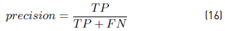
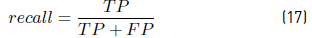
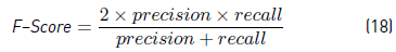
Relevant metrics were studied, including the precision of the prediction, recall (the conditional probability that the appliance is ON given that the prediction is ON); F-Score (the harmonic mean of precision and recall); the error of the total assigned energy consumption and the mean normalized error in assigned energy consumption.
Experimental results were processed using the available tools from the nilmtk toolkit, including the comparison of the proposed algorithm with two standard built-in methods of the toolkit: Combinatorial Optimization (CO) and Factorial Hidden Markov Model (FHMM).Results show that the proposed algorithm is able to achieve accurate results, accounting for an average of 0.95 on the F-score metric in the most complex problem instances and low error in assigned energy consumption. The proposed algorithm significantly outperformed both CO and FHMM in all problem instances studied.
The research reported in this article was developed within the project “Computational intelligence to characterize the use of electric energy in residential customers”, funded by the National Administration of Power Plants and Electrical Transmissions (Spanish: Administración Nacional de Usinas y Trasmisiones Eléctricas, UTE), the Uruguayan government-owned power company and Universidad de la República, Uruguay. The project proposes the application of computational intelligence techniques for processing household electricity consumption data to characterize energy consumption, determine the use of appliances that have more impact on total consumption, and identify consumption patterns in residential customers. Knowledge and results generated in the project will be helpful to conceive and design a specific automatic recommendation system that takes into account both the point of view of users and the electricity company.
This work extends our previous article Household energy disaggregation based on pattern consumption similarities [11], presented at II Ibero-American Congress on Smart Cities, Soria, Spain, 2019. The main contributions of this article are: i) a detailed description of the problem and the proposed algorithm; ii) an extended experimental analysis by including new instances that account for different periods between consecutive load records (10 and 15 minutes), in accordance with the available consumption data from UTE, in Uruguay; and iii) new problem instances including noise in the energy consumption records, in order to analyze the robustness of the proposed method for household energy consumption disaggregation.
The article is structured as follows. Section 2 presents the formulation of the problem addressed in the article, while Section 3 presents a review of the main related work. Section 4 describes the proposed algorithm for residential household energy consumption disaggregation, and Section 5 reports the experimental analysis over all the considered problem instances. Finally, Section 6 presents the conclusions and the main lines of future work.
2. The problem of energy consumption disaggregation
This section describes the problem of energy consumption disaggregation in residential households and its mathematical formulation.
2.1 Generic description of the energy consumption disaggregation problem
The problem consists of disaggregating the overall energy consumption of a household into the individual consumption of a given number of appliances. Energy disaggregation is a particular case of a classification problem. One of the most widely studied approaches considers a set of signatures for household appliances to solve the related classification problem. However, it is difficult to find the set of features to accurately describe each appliance, which can be applied to different houses and different consumption patterns [12].
2.2 Mathematical formulation of the energy consumption disaggregation problem
The mathematical formulation of the problem of energy consumption disaggregation considers the following elements:
A set of appliances available in a household A = {a i }, i = 1, . . . , m.
A period of time T, discretized in intervals t.
A function C: A × T →
gives the power consumption of each appliance in a given time interval t.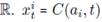
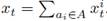
The aggregate power consumption of the household at a given time interval t, x t . The aggregate power consumption is expressed as the sum of the individual power consumption
of each appliance in use in that time interval .
.
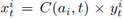
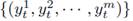
A binary variable
that indicates the status of appliance i in time interval t. takes the value 1 when
appliance i is ON and the value 0 when it is OFF.
The simplest version of the problem is the binary variant. It assumes two possible values for the power consumption of each appliance, i.e.,
 , that is to say, that the power consumption of appliance i is constant when switched on, and it does not depend on the activity being performed by the appliance.
The total power consumption is described as a function f:{0, 1} m → R defined by the expression in Equation 1 .

For those cases in which function f is injective (one-to-one), the problem is trivial. Otherwise, the times series {x t } t∈T must be studied, in order to learn and deduce from the variation of power consumption on time, the individual power consumption (or signatures) of the individual appliances.
Let us suppose an instance of the problem considering five appliances: fridge (power consumption 250 W), washing machine (power consumption 1500 W), dishwasher (power consumption 2250 W), kettle (power consumption 2000 W), and home theater (power consumption 80 W). For this set of appliances, the aggregate power consumption is a non-injective function. There is ambiguity between the power consumption of the fridge and kettle (combined) with the power consumption of the dishwasher, as defined by Equation 2. The variation of the aggregate power consumption in time must be studied to deduce if the dishwasher or the combination of fridge and kettle is ON.

Several attributes can be studied, and patterns can be detected to solve ambiguities. In the previous example, additional information can be used to solve the ambiguity: e.g., the mean time of utilization of each appliance (it is a couple of minutes for the kettle and more prolonged than an hour for the dishwasher).
Another more sophisticated patterns can be detected to solve problem instances with more complex ambiguities.
In general, the variation of the aggregated power consumption in a time neighbourhood of instant t can be used to deduce the configuration of all appliances
 with t∈T. The proposed approach is based on using the available information to make predictions
 with t∈T that maximizes the number of time intervals t∈T for which the status of every appliance is correctly detected; represented by the sum in Equation 3.
3. Related works
The analysis of the related literature allows identifying several proposals on the design and application of software-based methods for energy consumption disaggregation. This section reviews the main related works on this topic.
Hart presented the concept of Non-intrusive Appliance Load Monitoring in the pioneering publication on this research area [13]. The author stated that the previously presented approaches on the subject had a strong hardware component, installing intrusively monitoring points in each household appliance connected to a central information collector. These methods, in general, had the characteristic of relegating the software to the task of collecting data. Hart proposed an approach based on using simple hardware and sophisticated software for the analysis, therefore eliminating permanent intrusion in homes (i.e., the “non-intrusive” term was coined).
Hart defined a model for the analysis considering that electrical appliances are connected in parallel to the electrical network and that the power consumed is additive [Equation 4], where a i (t) represents the ON/OFF state of an appliance at time t.
Multiphase loads with p phases are modelled as vectors of dimension p where each component is the load in each phase. The total charge of the vector is the sum of the p components. P i is defined as a vector representing the power consumed by device i when it is turned on [Equation 5], where P(t) is the p-vector corresponding to time t, and e(t) represents the noise or the recorded error for time t.
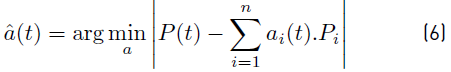
The proposed model involves solving a combinatorial optimization problem to determine vector a(t) from the known information., i.e., vectors P i and P(t), in order to minimize the error [Equation 6].
However, the resulting combinatorial optimization problem is NP-hard and therefore, computationally intractable for large values of n. Heuristic algorithms allow computing solutions of acceptable quality, but their applicability is limited because in practice the set of vectors P i is not fully known, the value n is not fixed, and unknown devices tend to be described as a combination of those already known. Furthermore, a small variation in the measurement of P(t) can cause significant changes in a(t), mistakenly predicting simultaneous ON and OFF events. In order to avoid these miss-predictions, Hart proposed the principle of continuity switch, establishing that for small intervals of time it is expected that few appliances have a change in their status (ON/OFF). Additionally, the principle assumes that no household appliance has a negative consumption in order to eliminate the ambiguity produced between the switch-on of a given appliance and the shutdown of an energy generator. For this reason, it is assumed that there are no electric generators connected to the network in the studied home.
In recent works, NILM has been treated as a machine learning problem, applying supervised and unsupervised learning methods to solve it. Supervised learning approaches are based on data sets of consumption of each device and the aggregate signal. The approach aims to generate models that learn how to disaggregate the signal of the devices from the aggregate signal. Most commonly techniques applied in this approach are Bayesian learning and neural networks. Unsupervised approaches seek to learn signatures of possible devices from the aggregate signal without knowing a priori what devices are inside the circuit.
As with all machine learning problems, it is essential to have measurement data in order to apply the different algorithms. Bonfigli et al. presented a survey of the test data sets available to researchers and the main techniques used for the unsupervised NILM approach [14]. The most used unsupervised learning techniques are those based on Hidden Markov Models (HMM), which define a number of hidden states in which the model can be moved, representing the operating conditions of the device (e.g., ON, OFF, and possible intermediate states) and an observable result, which depends on the real state that represents the analyzed consumption data.
Kelly and Knottenbelt analyzed three deep neural networks applied to the NILM problem along with its generalization when processing appliances not present on the training stage [15]. The proposed neural networks had between one and 150 million trainable parameters; therefore, large amounts of training data was needed. The data set used was UK-DALE, that records the total electricity consumption of five houses and its appliances. The work used a six-second sampling interval version of the dataset for the total and per-appliance electricity consumption, and limit the use of the appliances to five (fridge, washing machine, dishwasher, kettle, and microwave). Each appliance is present in at least three of the five houses, and their electricity consumption is heterogeneous, ranging from ON/OFF appliances (e.g., kettle) to multi-state appliances (e.g., washing machines, which have complex consumption patterns). Low-energy appliances were not taken into account since their consumption tends to be lost in the noise of the network. The approach consisted of training a neural network for each household appliance that processes a sequence of aggregate total consumption and returns the prediction of the power demanded by the associated appliance. Three neural networks architectures were studied: i) long short-term memory (LSTM) recurrent neural network, suitable for working with data sequences because of its ability to associate the entire history of the inputs to an output vector; ii) self-coding for noise elimination (denoising autoencoder, dAE) that cleans the aggregate consumption signal to obtain only the corresponding to the target appliance; and iii) rectangles network, which focuses on detecting the start and end of the use of the target appliance, and its average power demanded at that time. The networks were trained using 50% of real data and 50% of synthetic data, generated with the signatures of UK-DALE appliances. Results were compared with CO and FHMM. In the training stage (using training data), dAE outperformed CO and FHMM in all appliances regarding all metrics, except relative error in total energy. The rectangles network computed better results than CO and FHMM in all appliances, except the microwave, regarding all studied metrics. In the evaluation stage (using evaluation data), dAE and rectangles network outperformed CO and FHMM in F1 score, precision, proportion of total energy correctly assigned, and mean absolute error. LSTM network outperformed CO and FHMM in ON/OFF appliances but was behind in multi-state appliances.
Several related works have used the nilmtk tool, developed by Batra et al. nilmtk is a framework for NILM analysis implemented in Python that facilitates using multiple data sets by converting them to a standard data model [7].
Furthermore, nilmtk implements algorithms for data preprocessing, statistics to describe the data sets, disaggregation algorithms (such as CO and FHMM), and metrics to evaluate the performance of developed models. Preprocessing algorithms include downsample, to normalize the frequency of consumption signals; and voltage normalization, which implements a method to normalize the data and is able to combine different sets of household data to deal with the variation of voltage in different countries.
The REDD dataset was introduced to study the performance of the FHMM algorithm in the NILM problem [16]. The experimental analysis used two weeks of data from five households with ten-second sampling intervals. Results showed that FHMM classified correctly 64.5% of the consumption in the training set and 47.7% in the evaluation test. Although results are reasonable, it is evident their degradation between the training and the evaluation sets. The authors posed the challenge of combining REDD with the massive amount of untagged data generated daily by public energy companies.
4. The pattern similarities algorithm for energy disaggregation
This section describes the proposed algorithm to solve the problem of energy consumption disaggregation based on similar consumption patterns.
4.1 Algorithm description
The main details of the proposed algorithm are presented next.
Generic description
Function f: {0, 1} m → R gives the aggregate power consumption of a house for a set of appliances. A function g: R 2d+1 → R m is considered, where the positive number d determines a time neighbourhood for the predictions [Equation 7].

In Equation 7,
 is the estimated configuration of the set of house appliances. Function g
W,Z
has random elements; it is defined using the information of a training dataset {W,Z} = {w
t
, z
t
} such that for t = 1, · · · , n, w
t
∈ {0, 1}
m
, z
t
∈ R and Equation 8 holds.
is the estimated configuration of the set of house appliances. Function g
W,Z
has random elements; it is defined using the information of a training dataset {W,Z} = {w
t
, z
t
} such that for t = 1, · · · , n, w
t
∈ {0, 1}
m
, z
t
∈ R and Equation 8 holds.

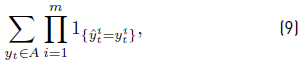
Parameters of function g W,Z are chosen empirically to maximize the sum in Equation 9, where A is the set of ambiguous configurations A = {y ∈ {0, 1} m /∃y′ ∈ {0, 1} m , y′ ≠ y, f(y′) = f(y)}, equivalent to maximize the number of time intervals t ∈ T for which every appliance status is correctly detected [Equation 3].
The output of the algorithm is ⃗y, the vector of disaggregated power consumption, computed using the following input:
• The vector X containing the aggregate power consumption of one house measured over a period with a certain time-frequency.
A training set Z containing the aggregate power consumption of one or several houses measured over a period with the same time-frequency as X.
A training set W containing the disaggregated power consumption of the house (houses) described in Z over the same period and with the same frequency as X is measured.
The parameter d that defines a time interval neighbourhood.
The parameter δ that defines a power consumption neighbourhood.
The parameter H that separates high from low power consumption.
The proposed algorithm, named Pattern Similarities (PS), consists of two parts, training and testing (prediction), described next.
Training Stage
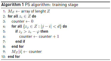
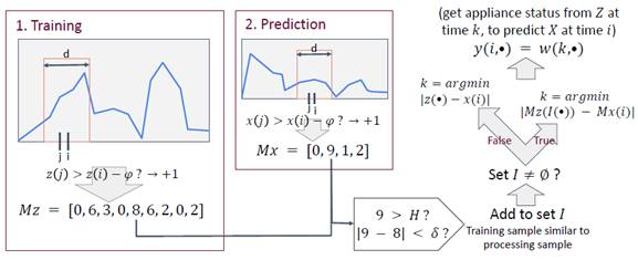
Algorithm 1 describes the training stage. This stage builds an array (M Z ), whose elements relate each consumption record on the training set to nearby records in the past and in the future. Each element of the array (z j ∈ M Z ) can be interpreted as the value of a feature of appliances signatures. The main loop (lines 2-10) iterates over each sample in the training dataset. In each iteration step, the algorithm counts how many consumptions from the time neighbour samples are similar to the consumption of the iteration step sample (nested loop in lines 4-8) . In line 9, the array (M Z ) is updated with the value of the counter, in the position corresponding to the consumption sample analyzed in the iteration. That array is used then, in the testing stage, to find samples whose consumption pattern is similar to the sample processed.
Testing Stage
Algorithm 2 describes the processing of the testing stage. The first loop (lines 1-10) is similar to the main loop of the training stage, but applied to the testing dataset. The result is an array M X , whose elements relate each consumption record on the testing set to nearby records in the past and in the future. The second loop (lines 11-27) iterates over each testing sample to find similarities with samples of the training dataset. The third loop (nested into the second, lines 13-17) compares each element of the array created in the training stage to the corresponding sample of the array created in the first loop. If the difference between elements is lower than threshold δ and the testing sample has a consumption greater than threshold H (δ and H defined in 4.1), a reference index of the training element is added to set I to be considered in next comparisons. Thus, two key elements of the problem, the energy consumption and its variation in a time neighbourhood, are used in the disaggregation process.
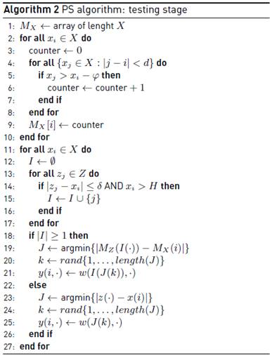
If the set I has elements, the samples that minimize the difference between signature features (the difference between M Z and M X ) are selected. The minimum of the vector |M Z (I(·)) − M X (i)| is not necessarily attained at a single sample, thus line 19 defines set J with the indexes where the minimum is attained. In line 20, one index of the set J is randomly chosen. If set I is empty, i.e., no training sample similar to the processing sample was found, the algorithm selects the training samples that minimize the difference of consumption with the sample that is being processed (line 23). The reference indexes of the selected samples are stored in the set J (line 23), and one of them is chosen (line 24). Once the algorithm has found a similar training sample, its reference index is related to the appliance states (ON/OFF) at the time of the record (line 21 or 25, depending on I).
Figure 1 graphically summarizes the stages of the proposed PS algorithm.
4.2 Implementation
A first version of the proposed algorithm was developed on Matlab, version 8.3.0.532 (R2014a), as a proof of concept. After that, the PS algorithm was re-implemented on python version 3, using pandas and numpy, which allows the implementation to be included as part of a pipe of execution in nilmtk. For this stage, several modifications were included in the metrics and utils files of the framework.
Two scripts were implemented for generating the synthetic datasets. The first script reads the UK-DALE dataset (HDF5 file), normalizes the values for houses and appliances, and builds a directory structure that contains metadata and the normalized data in CSV files. The normalization replaces all records over a given threshold by an indicated value, and set all other values to zero. For the generation of instances that include noise, the script executes a function that adds power consumption of extra appliances, whose behaviour is modelled as exponential probability models (see details in Subsection 5.3).
The second script reads the directory structure and its content to generate a new HDF5 file with the synthetic dataset. In the resulting dataset, data have the same sample rate than in the original dataset. The algorithm implementation, the scripts for generating the datasets, and the modified nilmtk files are available on a public repository (gitlab.com/jpchavat/nilm-scripts).
5. Experimental analysis
This section presents the experimental analysis of the proposed PS algorithm. The algorithm was executed in a nilmtk pipeline of execution, using a synthetic dataset based on UK-DALE dataset as input. The disaggregation accuracy was studied considering different sample intervals, in order to analyze possible degradations when considering few available data (i.e., larger sample intervals), and considering ambiguous appliance loads and noise in the signals, in order to analyze its robustness. Results of the PS algorithm were compared with the results of CO and FHMM algorithms executed in the same settings.
5.1 Datasets and problem instances
This subsection describes the datasets and problem instances considered in the experimental evaluation.
Datasets
Datasets used in the experiments were synthetically generated based on real data from house #1 of the UK-DALE dataset. Data for the following appliances were considered: fridge, washing machine, kettle, dishwasher, and home theatre. These appliances are representative of devices that contribute the most to household energy consumption [17]. Several python scripts were generated for instances generation. The tools of the nilmtk framework, and the pandas and numpy libraries were used along the process.
The instances of the datasets were generated according to the following procedure:
Python scripts are used for reading UK-DALE data structure and creating own metadata, following the structure of NILM-Metadata proposed by Kelly and Knottenbelt [18].
Two types of values were used for the normalization. In one case, the mean of the maximum current consumption of each activation is computed for each appliance. In the other case, a list of constant values was set for the normalization.
Each record in the UK-DALE dataset that is over a given threshold (set to 5.0 W) is transformed, normalizing it using the values previously calculated, i.e., if the record corresponds to a power consumption above 5.0 W, it is replaced by the values calculated/defined in step two, if not, it is replaced by zero.
The resulting datasets have the same sample rate than the original UK-DALE dataset, with the particularity that it does not present gaps, i.e., if the original sample rate is six seconds, the generated dataset will have strictly one record every six seconds with zeros filling the gaps presented in the original dataset.
The applied methodology for generating problem instances is generic and allows creating data for every building and every appliance. It can be used over base data from the UK-DALE dataset or other similar datasets from repositories in the literature.
Problem instances
Five different base instances were generated for the experimental analysis: instances #1 to #3 by downsampling the UK-DALE dataset to an interval of 5 minutes and instances #4 and #5 by downsampling the UK-DALE to intervals of 5, 10, and 15 minutes (see details in Section 5.2). A datetime range limit was established for training and testing data. For training data, the limits were set from 2013-01-01 at 00:00:00 to 2013-07-01 at 00:00:00, while for the testing data, the limits were set from 2013-07-01 at 00:00:00 to 2013-12-31 at 23:59:59. A threshold of minimum consumption (H) was applied in the normalization, which was set to 5.0 W. This threshold allows discarding standby power consumption records.
The first four instances were generated to analyze the efficacy of the proposed algorithm to solve different cases of energy consumption ambiguity. The fifth instance, apart from the presence of ambiguity, includes noise signals of appliances that are not intended to be disaggregated.
A description of each problem instance and the motivation of using it is provided next.
Instance #1. The generated dataset normalizes the consumption of each appliance using the value of the median of maximum consumption per activation (i.e., periods in which an appliance remains in state ON). Outliers were filtered by lower and upper limits defined by the standard deviation. The generated dataset is used for training and testing the algorithms. This instance aims at working with values close to the real ones but keeping constant consumption values over time.
Instance #2. The generated dataset normalizes the consumption values to generate ambiguity between the consumption of two appliances: kettle and dishwasher. The same dataset is used for training and testing the algorithms. This instance aims at testing how the algorithms solve the most basic case of ambiguity.
Instance #3. The generated dataset normalizes consumption values in a similar way than instance #2, but in this case including ambiguities between the sum of consumption of three appliances (fridge, home theatre, and washing machine) with the consumption of another appliance (dishwasher). The same dataset is used for training and testing the algorithms. This instance aims at studying how the algorithms solve a more sophisticated case of ambiguity.
Instance #4. The training dataset is the same than in instance #2; but a new dataset was generated for the testing stage, introducing small variations in the consumption of every appliance, but the washing machine. For example, the consumption of the fridge was normalized to 260 W instead of 250 W. This instance was designed to evaluate the proposed algorithm in a scenario where testing appliances are similar but not equal to the appliances used for training.
Instance #5. The dataset takes as a base the testing dataset of the instance #4 and adds the consumption of extra appliances to simulate noise in the signal. The behaviour of each extra appliance is modelled as a discretization of an exponential variable, procedure explained in Subsection 5.3. This instance aims to analyze the robustness of the algorithm in the presence of unknown power consumption values.
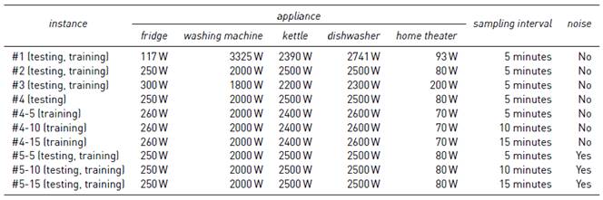
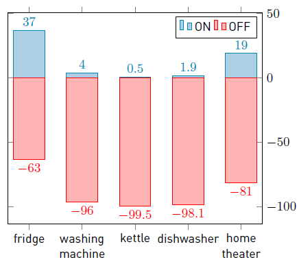
Table 1 reports the normalized power consumption values for each appliance, the sampling intervals, and the presence of noise used for training and testing in each instance. In turn, Figure 2 shows the percentage of records when each appliance is in state ON/OFF, which is the same for all the generated datasets. Values were obtained by applying data analysis to the UK-DALE dataset.
Table 1 Instances of datasets: normalized consumption of appliances, sampling intervals, and the presence of noise
5.2 Analysis of different sampling intervals
Instances #4 and #5 have three sub-instances (each) that vary the sampling interval, i.e., the period between two consecutive power consumption records: 5 minutes (sub-instances #4-5 and #5-5 ), 10 minutes (sub-instances #4-10 and #5-10) and 15 minutes (sub-instances #4-15 and #5-15). Instances with different sampling intervals are conceived to evaluate the proposed PS algorithm in scenarios where the available data is more disperse in time, closer to the real scenarios available by the national electric company (UTE).
5.3 Adding noise to model uncertainty
Instance #5 include extra appliances, not considered in previous instances, which are not intended to be disaggregated. Instead, they are used to add noise to the aggregated consumption signal. The main goal of including those appliances is analyzing the robustness of the proposed approach under the presence of uncertain power consumption data. The procedure for generating the consumption of an extra appliance is as follows.
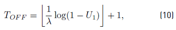
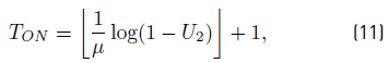
Switching on and off a given appliance is assumed to be a Poisson point process, i.e., they occur continuously and independently at a nearly constant average rate. The time interval in which the appliance status is OFF (T OFF ) is assumed to be a discretization of an exponential distribution of parameter λ and the time interval in which the appliance status is ON (T ON ) is assumed to be a discretization of an exponential distribution of parameter μ [Equations 10-11], where U 1, U 2 are random numbers with uniform distribution in [0, 1] and ⌊x⌋ stands for the integer part of x.
The procedure applied to generate noise for a single appliance is described in Algorithm 3.
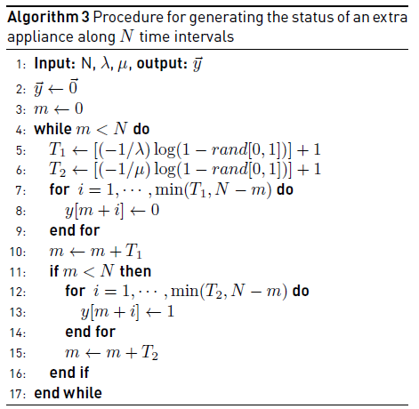
The procedure in Algorithm 3 works as follows. The output vector ⃗y is initialized as a vector of zeros of length N. The main loop iterates until generating N time intervals. T
1 represents a realisation of variable T
OFF
, generated using the distribution defined in Equation 10 (line 5). Variable
 has exponential distribution with parameter λ and T
OFF
has geometric distribution with parameter 1 − e
−λ
[19]. T
2 represents a realisation of variable T
ON
that has a geometric distribution with parameter 1 − e
−μ
, generated using the distribution defined in Equation 11 (line 6).
has exponential distribution with parameter λ and T
OFF
has geometric distribution with parameter 1 − e
−λ
[19]. T
2 represents a realisation of variable T
ON
that has a geometric distribution with parameter 1 − e
−μ
, generated using the distribution defined in Equation 11 (line 6).
In lines 7-9, the OFF period of the appliance is added to the noise generated so far (components equal to zero). The case in which the number of time intervals simulated so far is greater than the desired length N is contemplated by the expression min (T 1 , N − m). In line 10, the value of m is modified according to the number of zeros added in lines 7-9. If the value of m is smaller than N, the ON period of the appliance is added to the noise generated so far (components equal to one) (lines 12-14). The case in which the number of time intervals simulated so far is greater than the desired length N is contemplated by the expression min (T 2 , N − m).
Table 2 Description of the appliances included in the problem instances to simulate noisy loads. ST is the sampling time expressed in seconds
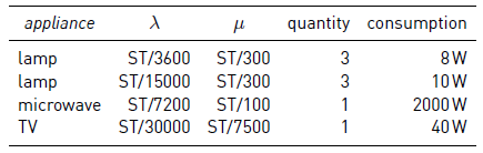
A series of zeros and ones is then generated for each extra appliance, according to the values of parameters λ and μ reported in Table 2 and the noise in the form of aggregate power of these extra appliances is calculated according to their power consumption values. For instance, for an interval of 5 minutes and three lamps of 8 W, λ = 300/3600 implies that the mean time OFF for these appliances is (1 − e −λ ) −1 ≈ 12.5 intervals of 5 minutes, i.e., approximately 62 minutes and the mean time ON is (1 − e −μ ) −1 = (1 − e −1 ) −1 ≈ 1.58 intervals of 5 minutes, i.e., approximately 8 minutes. The same computation for lamps of 10 W results in a mean time OFF of 4 hours and 12 minutes. Similarly, λ = 1/100 gives a mean time OFF for the TV set of 8 hours and 22 minutes and μ = 1/25 gives a mean time ON of 2 hours and 7 minutes. Finally, λ = 1/24 gives a mean time OFF for the microwave of 2 hours and 2 minutes and μ = 3 gives a mean time ON of 5 minutes. The fact that the values of λ and μ are proportional to the length of the sampling intervals gives similar ON and OFF mean values for the 10 and the 15 minutes sample.
In summary, for each sample interval, noise is generated in the form of seven low consumption appliances (six lamps and one TV set) and one high consumption appliance (microwave), according to Algorithm 3 and Table 2. Sub-instances #5-5, #5-10 and #5-15 are formulated to evaluate PS algorithm in scenarios where there are appliances apart of the ones to be disaggregated. In real scenarios, it is not reasonable to assume that two different houses have identical sets of appliances. Additionally, it is not possible to measure all appliances of a house separately, and the consumption of the appliances not included in the set of interest could be considered as noise in the context of the problem. These facts justify the inclusion of such sub-instances in order to get a more real problem.
5.4 Software and hardware platform
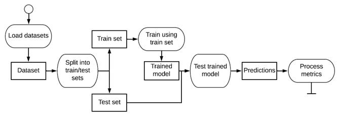
The nilmtk framework was used to implement a pipeline of execution for the experiments, as described in Figure 3.
The first stage of the pipeline loads the dataset while the second split the dataset into a training set and a testing set. The training set is used to train the algorithm in its different instances and then the testing set is used to obtain the results of disaggregation. Finally, results are compared with the ground truth data (i.e. the test set) to compute a set of metrics.
The experimental evaluation was performed on National Supercomputing Center (Cluster-UY) infrastructure that counts with Intel Xeon-Gold 6138 nodes (up to 1120 CPU cores), 3.5 TB RAM, and 28 GPU Nvidia Tesla P100, connected by a high-speed 10 Gbps Ethernet network (cluster.uy) [20].
5.5 Baseline algorithms for comparison
Two methods from the related literature were considered as baseline for the comparison of the results obtained by the proposed algorithm: CO and FHMM.
The CO method was first presented by Hart, and included in the nilmtk framework. The approach of CO is to find the optimal combination of appliance states that minimises the difference between the total sum of aggregated consumption and the sum of the consumption of the predicted state on of appliances. CO searches for a vector
 that minimises the expression on Equation 6 Given the complexity of the CO algorithm, which is exponential in the number of appliances, it is not useful to address scenarios with a large number of appliances. The complexity of the CO algorithm is exponential in the number of appliances. Thus, it is not useful to address scenarios with a large number of appliances.
After the introduction of FHMM [21], different variations were developed to solve the energy disaggregation problem [22]. HMM are mixture models that encode historical information of a temporal series in a unique multinomial variable, represented as a hidden state; FHMM extends HMM to allow modeling multiple independent hidden state sequences simultaneously. FHMM scales worst than CO in scenarios with a large number of appliances, due to the inherent computational complexity of the method.
5.6 Metrics for results evaluation
A set of standard metrics were applied to evaluate the efficacy of the proposed PS and baseline algorithms. Consider that
 is the actual status series for appliance n and
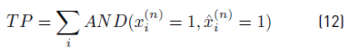
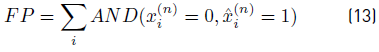
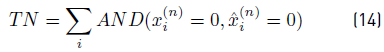
 the status series predicted by the algorithm. Then, True Positive (TP), False Positive (FP), True Negative (TN), and False Negative (FN) ratios are defined by Equations 12-15.
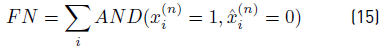
Five metrics are considered in the analysis:
precision of the prediction, defined as an estimator of the conditional probability of predicting ON given that the appliance is ON [Equation 16].
recall, defined as the conditional probability that the appliance is ON given that the prediction is ON [Equation 17].
F-Score, defined as the harmonic mean of precision and recall [Equation 18].
Error in Total Energy Assigned (TEE), defined as the error of the total assigned consumptions [Equation 19].
Normalized Error in Assigned Power (NEAP), defined as the mean normalized error in assigned consumptions [Equation 20].
5.7 Results
This subsection reports the numerical results of PS and the baseline CO and FHMM algorithms in the experimental evaluation. Regarding PS, all results were obtained using the following parameter configuration, set by a rule-of-thumb and empirical evaluation: δ = 100, d = 10, H = 500 and φ = 250.
Instances without noise and sampling interval of 5 minutes
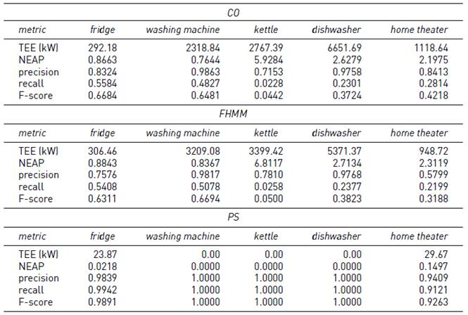
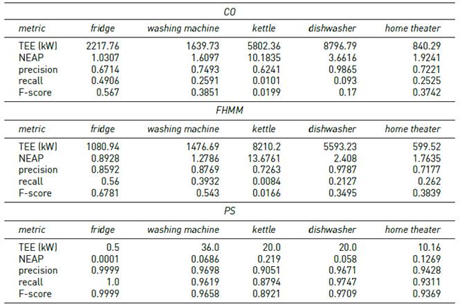
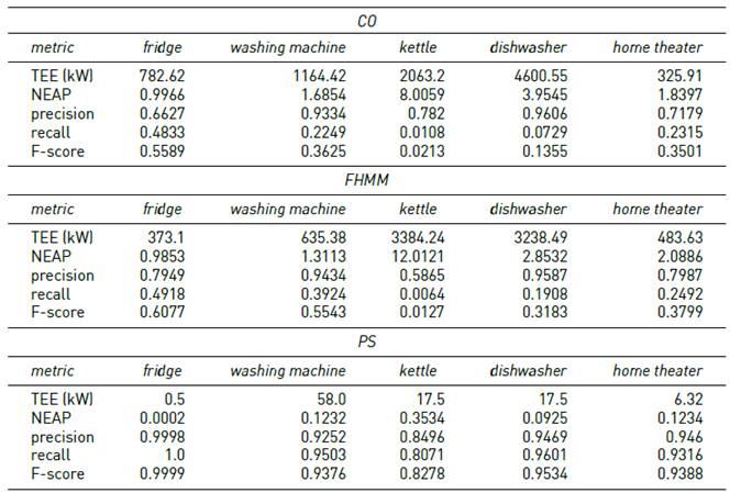
Tables 3-6 report the results of the proposed algorithm (PS) and the baseline algorithms (CO and FHMM), on instances #1 to #4, considering a period of 5 minutes between consecutive energy consumption records.
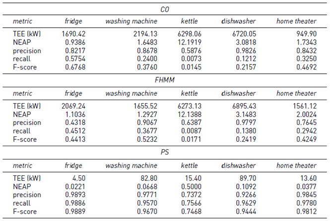
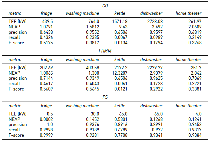
Results in Table 3 indicate that PS was able to accurately solve problem instances without ambiguity between the power consumption of appliances. F-score values between 0.92 and 1.0 were obtained. Both CO and FHMM got F-score values around 0.6 for fridge and washing machine, around 0.3 for dishwasher and home theater, and 0.04 (i.e., almost null) for kettle. In all cases, F-score values were lower than the obtained with PS.
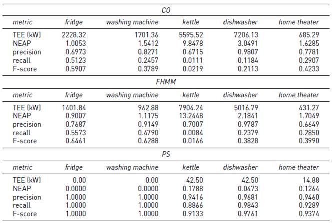
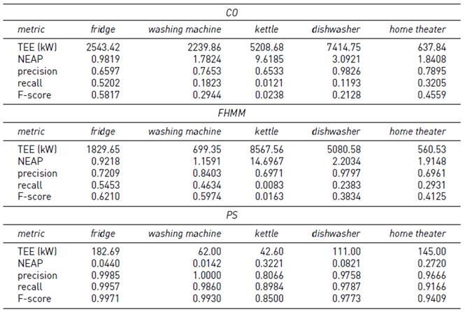
Results in Table 4 indicate that F-score values obtained by PS for appliances with ambiguities decreased up to 9%, while the rest of the F-score values remains similar to instance #1. Regarding the baseline algorithms, CO showed a decrease of 50% in the prediction of appliances with ambiguity, while results of FHMM remained similar to the ones computed for instance #1, except for the kettle (F-score value decreased 66%).
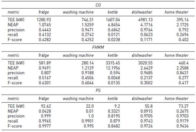
Results in Table 5 indicates that the F-score values of PS decreased for washing machine (3%), dishwasher (6%), and kettle (the worst value, 25% less than for instance #1). On the other hand, F-score values increased for home theatre (6%) and did not vary for the fridge. F-score values of the CO algorithm decreased for washing machine (42%), kettle (67%), and dishwasher (42%), compared with instance #1. In turn, F-score values for FHMM decreased for all the appliances (up to 66% for kettle), but the home theatre (increased 33%).
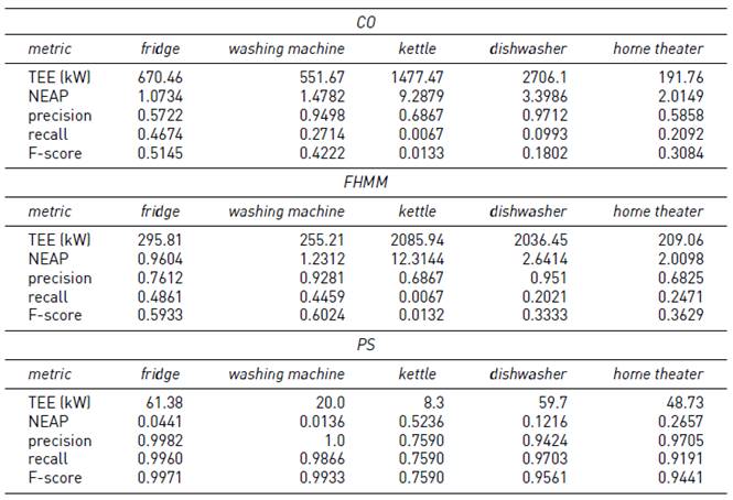
Finally, results in Table 6 demonstrate that the proposed PS algorithm has a robust behaviour when using different normalized datasets for training and testing steps, which slightly differ in the power consumption values used in the normalization. The F-score for PS was greater than 0.99 for fridge and washing machine, greater than 0.97 for dishwasher, and greater than 0.94 for home theatre. The lowest F-score value was obtained for the kettle (0.85), which, similarly to instances #2 and #3, had the lowest F-score values among all appliances. For instance #1, the F-score of the kettle decreased 15%. The rest of the appliances experienced a decrease/increase lower than 2%. In the case of the CO algorithm, concerning instance #1, the F-score decreased 13% for the fridge, 55% for the washing machine, 46% for the kettle, and 43% for the dishwasher. In the case of the home theatre, the F-score increased 8%. For the FHMM algorithm, F-score values of fridge and dishwasher varied less than 1.6% with respect to instance #1, and decreased for washing machine (11%) and kettle (67%).
Instances without noise and variable sampling interval
Tables 6-8 report the results of the PS, CO, and FHMM algorithms on instances #4-5, #4-10 and #4-15, where the sampling interval varies in 5, 10 and 15 minutes.
In the case of the F-score of the PS algorithm, the results show a decrease of 10.5% for the appliance kettle from the 5 minutes sampling interval to the 15 minutes version, while in the other appliances the decrease is below 2.2%. Concerning to the TEE and NEAP metrics, the results of the algorithm PS remain below 183 kW and 0.52 respectively. In general, the F-score of both CO and FHMM algorithms remained lower than the F-score of PS. Compared with the results varying the sampling intervals, the results are mixed. The CO algorithm was able to improve up to 70% in the case of the washing machine, but it reduced more than 50% in the case of the kettle. The F-score of the FHMM algorithm remained similar along the three instances, with no variations or variations below 10%. The TEE for both CO and FHMM algorithms decreased in general, up to a decimal part in some cases, while the NEAP metric varied up to 20% increasing or decreasing.
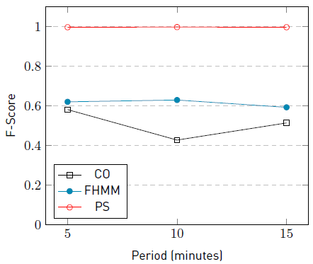
The graphics in Figure 4 and Figure 5 summarize the F-score results of the three studied algorithms in the three variations of the sampling intervals for the appliances fridge and kettle, respectively. The fridge was selected for the graphic because it presents the longest activation time, while the kettle was selected because it presents the shortest activation time. Overall, results of the PS algorithm were always better than those computed by CO and FHMM. Furthermore, PS results show high robustness, even when dealing with long sampling intervals.
Instances with noise and variable sampling interval
Tables 9-11 report the result of PS, CO, and FHMM on instances #5-5, #5-10 and #5-15. In these instances, apart of varying the sampling interval in 5, 10 and 15 minutes, the consumption of extra appliances to generate noise in the signal is added.
Regarding the F-score metric of the PS algorithm, the comparison of instances #5-5 (smaller sampling interval) and instance #5-15 (larger sampling interval) indicates that the results decreased up to 13% for washing machine, kettle, and dishwasher, while F-score remained similar for fridge and home theatre. Values of TEE and NEAP metrics were all above 65kW and 0.53 respectively, disregarding the appliance.
In the three sub-instances studied, the F-score of the PS algorithm was higher than the F-score of CO and FHMM. In addition, PS presented lower values than CO or FHMM for TEE and NEAP, in all cases. The F-score of CO decreased 9% (for fridge) and 13.5% (for home theatre), and did not vary for other appliances. TEE decreased up to one third for all appliances, while NEAP presented similar values. F-score for FHMM decreased up to 17% in all appliances but the washing machine (incremented 3.5%). TEE decreased up to one fifth in all appliances, and NEAP remained similar.
When comparing the results for all sub-instances of instances #4 and #5 (i.e., lack of noise vs. presence of noise), the results of the PS algorithm are different depending on the sub-instance:
#4-5 vs #5-5: the F-score for the washing machine and home theatre decreased up to 3%. On the other
#4-5 vs #5-5: the F-score for the washing machine and home theatre decreased up to 3%. On the other hand, the F-score increased 4.5% for the kettle and remained equal for the other appliances. Concerning TEE and NEAP, both metrics reduced their values when comparing sub-instance #4-5 with #5-5.
#4-10 vs #5-10: the F-score for washing machine, kettle, dishwasher, and home theatre decreased from 0.5% up to 9.1%, while did not vary for fridge. Regarding TEE, the values decreased for all appliances but the kettle. Results for the NEAP metric showed values lower than 0.35 in both instances, for all appliances.
#4-15 vs #5-15: the F-score for appliances washing machine and dishwasher decreased up to 6.5%, while it increased up to 1.4% for the kettle and home theatre. F-score values for the fridge remained similar between instances. For TEE, results decreased for the fridge and increased for the other appliances, maintaining in all cases values below 62kW. The NEAP metric results show similar values for both instances.
The F-score of the algorithm PS for the Washing machine decreases in the three sub-instances with the presence of noise. Similarly, a decrease in the F-score was recorded in two of the three sub-instances for the appliances washing machine and dishwasher. In the other hand, fridge kept similar values than in sub-instances without noise (i.e., instance #4) while the kettle increases its F-score in two of the three sub-instances. Results in sub-instances with the presence of noise show a tendency to decrease the performance in appliances with a low number of activations and long activation times, in the presence of noise and increasing sampling intervals.
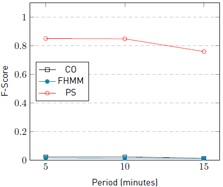
The graphic in Figure 6 summarizes the F-score results of the algorithms CO, FHMM, and PS for the appliance fridge in the problem instances #5-5, #5-10, and #5-15. The graphic in Figure 7 summarizes the F-Score of the algorithms for the appliance kettle in the same scenarios.
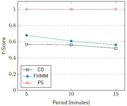
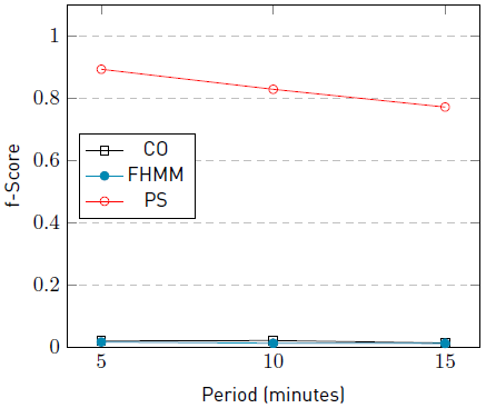
Results of PS in Figures 6 and 7 show that the appliance fridge, which presents the highest number of activations, remains unchanged along with the instances. In contstrast, results for CO and FHMM decrease along with the instances. On the other hand, the results of PS for the appliance kettle, which presents the lowest number of activations, shows that the F-score decrease as the sampling interval increases. It is expected to observe the same behaviour for the algorithms CO and FHMM, but the resulted F-score values are too low to conclude.
The reported results suggest that the presence of extra appliances that generate noise in the aggregated signal decrease the F-score performance of the PS algorithm in most cases and up to 9.1%. The decrement of F-score for PS is observed more frequently in appliances with lower activation time than in ones with high activation times. For CO and FHMM, results suggest that the F-score decrease independently of the activation time. In general, results indicate that in the presence of noise, as the sampling interval increases, the F-score performance is degraded up to 13%.
Summary
Overall, the proposed PS algorithm achieved satisfactory results for all the studied instances of the power consumption disaggregation problem.
Regarding the F-score metric, for instances without noise and fixed sampling intervals of 5 minutes, improvements of PS were 60% over CO and 57% over FHMM in average, and up to 64% over CO in problem instance #4-5 and up to 60% over FHMM in problem instance #3. When considering different sampling intervals, improvements were 69% over CO and 59% over FHMM on average, and up to 98% over CO and FHMM in problem instances #4-15 and #4-5, respectively. For instance #4-15, with the maximum sampling interval, results improved between 48% (worst case) and 98% (best case), with an average improvement of 70%, over CO. Similar results were obtained when comparing with FHMM: PS results improved 98% in the best case, 60% on average, and 39% in the worst case. In problem instances with noise and different sampling intervals, PS improved over baseline CO results up to 98% in the best case (instance #5-15), 69% in average, and 43% in the worst case (instance #5-5). For baseline FHMM results, PS improved up to 98% in the best case (the three sub-instances), 61% on average, and 32% in the worst case (instance #5-5). For instance #5-15, improvements of PS ranged from 39% to 98% over CO and from 48% to 98% over FHMM.
Furthermore, PS systematically obtained the lowest values of both TEE and NEAP for all instances. The degradation of results obtained for the kettle in problem instances with ambiguity, long sampling periods, or noise, suggest that the lower percentage of operating time (0.5% of the total time in ON state) negatively affects the results. The more complex the dataset is, the more consumption data are needed in the testing dataset, especially to capture the ON/OFF behavior of appliances with shorter operating time.
The graphics in Figures 8 and 9 summarize the F-score obtained by CO, FHMM and PS algorithms for all studied instances with a sampling interval of 5 minutes for fridge and washing machine, respectively. These appliances were selected because they present the larger (fridge) and mean (washing machine) activation time. In all the scenarios, PS obtained considerably better results than the baseline algorithms.
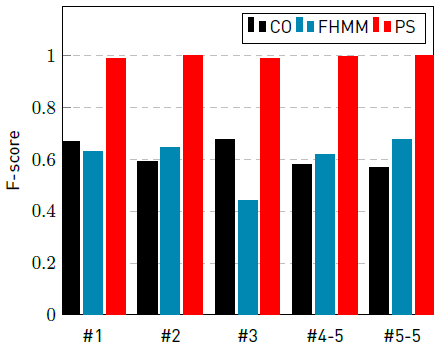
Figure 8 F-score of CO, FHMM, and PS for instances with a sampling interval of 5 minutes, for appliance fridge
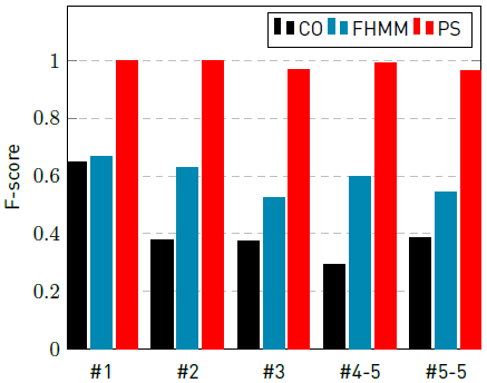
Figure 9 F-score of CO, FHMM, and PS for instances with a sampling interval of 5 minutes, for appliance washing machine
6. Conclusions and future work
This article presented a proposal to address the problem of household energy disaggregation using a non-intrusive approach. The PS algorithm, based on detecting pattern similarities between power consumption, was proposed. The method works in two stages: the training stage, that creates the data used to find pattern similarities; and the testing stage, that looks for patterns similarities between the training data and the data to be disaggregated.
The experimental evaluation was performed over realistic problem instances that consider the presence of ambiguous appliance consumptions, different sampling intervals, and extra appliances consumptions that are not intended to be disaggregated but modify the aggregate signal. Results were compared with two baseline algorithms, CO and FHMM, from the related literature.
PS achieved very satisfactory results, significantly outperforming CO and FHMM, with improvements in the F-score up to 64% for instances #1-#4-5, up to 69% for sub-instances of instance #4 and up to 98% for sub-instances of instance #5.
Overall, the obtained results showed that the proposed PS algorithm is effective for addressing the problem of energy consumption disaggregation. The proposed approach can be applied in practice as the first step for household energy planning by using intelligent recommendation systems [23].
The main lines for future work are related to performing an in-depth study of the training parameters of the proposed algorithm, in order to capture those patterns that currently are not learnt due to uncertainty or insufficient information available to solve ambiguities. Furthermore, the proposed approach must be extended by including the study of instances with the presence of multi-state or continuous variable appliances. The proposed methods can also be integrated into more sophisticated computational intelligent methods (e.g., long-short term memory neural networks) to solve the problem.

